Download
1 / 41
460 likes | 1.14k Views
Math Review with Matlab:. Fourier Analysis. Fourier Transform. S. Awad, Ph.D. D. Cinpinski E.C.E. Department University of Michigan-Dearborn. Fourier Transform. Energy Signal Definition. Motivation For Fourier Transform. Fourier Transform Representation. Example: FT Calculation.

E N D
Math Review with Matlab: Fourier Analysis Fourier Transform S. Awad, Ph.D. D. Cinpinski E.C.E. Department University of Michigan-Dearborn
Fourier Transform • Energy Signal Definition • Motivation For Fourier Transform • Fourier Transform Representation • Example: FT Calculation • Example: Pulse • Inverse Fourier Transform • Fourier Transform Properties • Example: Convolution • Parseval’s Theorem • Relation between X(s) and X(j) • Example: Ramp Function
Motivation for Fourier Transform We need a method of representing aperiodic signals in the frequency domain. The Fourier Series representation is only valid for periodic signals. The Fourier Transform will accomplish this task for us. However, it is important to note that the Fourier Transform is only valid for Energy Signals.
What is an Energy Signal ? A signal g(t) is called an Energy Signal if and only if it satisfies the following condition.
Fourier Transform Representation The Fourier Transform of an Energy Signal x(t) is found by using the following formula. There is a one to one correspondence between a signal x(t) and its Fourier Transform. For this reason, we can denote the following relationship.
x(t) = e-atu(t) 1 a > 0 t Example: FT Calculation • Note: If a<0, then x(t) does not have a Fourier transform because:
Fourier Transform complex function of w
Magnitude Response Let us now find the Magnitude Response. The expression for the magnitude response of a fraction is calculated as follows.
Magnitude Response Now calculate the Magnitude Response of X(j)
w (rad/sec) Magnitude Response We can now plot the Magnitude Response. Even function of w
Phase Response The expression for the phase response of a fraction is calculated as follows.
w(rad/sec) Phase Response We can now plot the Phase Response. Odd function of w
FT FT FT FT Fourier Transform Tables We could go ahead and find the Fourier Transform for any Energy Signal using the previous formula. However, Signals & Systems textbooks usually provide a table in which these have already been computed. Some are listed here.
x(t) 1 t -T1 T1 0 Example: Pulse • Find the Fourier Transform of:
Magnitude Response • Note: X(jw) = 0, when So:
Magnitude Response We can now plot the Magnitude Response.
Phase Response We can now plot the Phase Response.
Inverse Fourier Transform Recall that there is a one to one correspondence between a signal x(t) and its Fourier Transform X(j). If we have the Fourier Transform X(j) of a signal x(t), we would also like be able to find the original signal x(t).
Inverse Fourier Transform • Let X(jw) = FT{x(t)} = • x(t) = FT-1{X(jw)} = • FT-1 is the inverse Fourier Transform of X(jw)
Fourier Transform Properties There are several useful properties associated with the Fourier Transform: Time Domain Differentiation Property Linearity Property Time Scaling Property Time Domain Integration Property Duality Property Time Shifting Property Symmetry Property Frequency Shifting Property Convolution Property Multiplication by a Complex Exponential
Linearity Property Let: Then:
Time Scaling Property Let: where a is a real constant Then:
Duality Property Let: Then:
Time Shifting Property Let: • Note: “a”can be positive or negative Then:
Frequency Shifting Property Let: Then:
Time Domain Differentiation Property Let: Then:
Symmetry Property • If x(t) is a real-valued time function then conjugate symmetry exists: • Example:
Convolution Property Let: Convolution Then:
h(t) LTI System x(t) y(t) Convolution Example: Convolution Filter x(t) through the filter h(t) where h(t) is the impulse response
Example: Convolution Knowing We can write Note:
Multiplication by a Complex Exponential Let: Then:
Amplitude Modulation Sinusoid Examples (i)
Amplitude Modulation Sinusoid Examples (ii)
y(t)=x(t)cos(wot) x(t) X y(t) x(t) t t cos(wot) FT FT-1 Y(jw) X(jw) 1 w -wo wo w Amplitude Modulation
Time Domain Frequency Domain Parseval’s Theorem • Let x(t) be an energy signal which has a Fourier transform X(jw). • The energy of this signal can be calculated in either the time or frequency domain:
Frequency Response Relation between X(s) and X(jw) • If X(jw) exists for x(t): assuming x(t) = 0 for all t < 0 • Example: • H(s) is known as the transfer function
t Example: Ramp Function The Fourier Transform exists only if the region of convergence includes the j axis. To prove this point, let us look at the Unit Ramp Function. The Ramp Function has a Laplace Transform, but not a Fourier Transform.
The Laplace Transform is and the corresponding Region of Convergence (ROC) is Re(s) > 0 Example: Ramp Function If we define the Step Function as: The Unit Ramp Function can now be rewritten as t*u(t) Since the ROC does not include the j axis, this means that the Ramp Function does not have a Fourier Transform