Download
1 / 19
190 likes | 206 Views
A study on classifying oceanic environments based on biological and temporal factors, with a focus on Steller sea lions. The approach is adaptable and quantitative, considering spatial and temporal variability. The method involves data analysis using clustering algorithms. Results show shifts in oceanic regimes over time, impacting biological distributions. The study offers insights into seasonal and regime variabilities, aiding in understanding oceanic structures.

E N D
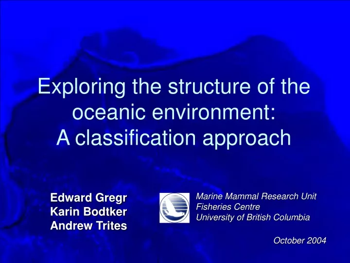
Exploring the structure of the oceanic environment: A classification approach Edward GregrKarin BodtkerAndrew Trites Marine Mammal Research Unit Fisheries Centre University of British Columbia October 2004
Why classify oceanic structure? • related to biological spatial distributions • temporal changes (e.g. regime shifts) • Steller sea lion in an ecosystem context
Extending the classification approach • biological perspective • quantitative and repeatable • adaptable • consider temporal variability (seasons, years, regimes) • different spatial scales (zooplankton vs. fish vs. sea lions)
High density Residential Industrial Roads Water Pasture Forest Wetland Grass A quantitative approache.g. classifying landscapes
Wind stress SSH Surface current speed SST SSS Data for oceanic classification 1 degree ROMS output1, interpolated to equal area grid. Seasonal averages,1966-1975 and 1980-1989. 1Yi Chao, Jet Propulsion Lab, California Institute of Technology
Sea surface salinity 33 31 32 34 35 0.0 -0.1 -0.2 -0.3 Sea surface temperature oC -0.4 -0.5 -0.6 -0.7 -0.8 + + + + + Classification methodH - means clustering algorithm1 Identify initial clusters Assign pixels to ‘nearest’ cluster based on maximum likelihood Iterate until stable 1Hartigan, J. A. 1975. Clustering Algorithms. John Wiley & Sons, New York.
60° 50° 40° 130° 30° 140° 150° 130° 180° 160° 170° 170° 160° 150° 140° Results: summer, 1966-1975
Results: correspond to domains Summer, 1966-1975
60° Pre - winter Post - winter 50° 40° 130° 30° 140° 150° 130° 180° 160° 170° 170° 160° 150° 140° Results: regime variability • Alaska gyre: evidence of stronger flow post - 1976 • Transitional domain: boundary shift
Post-76 Pre-76 Winter Spring Summer Fall • Consistency between some seasons differs before and after regime shift Results: map comparisons • Seasons more similar between regimes than consecutive seasons within each regime
1.38 0.70 1.03 0.41 0.56 Results: biological relevance Chl-a, mg/L1 Summer, 1997-2003 1Andrew Thomas, School of Marine Sciences, University of Maine
Summary • quantitative and adaptable approach • regions correspond to classic domains • temporal differences mapped and quantified • regions have biological relevance
Thanks very much ... Intellectual:Ian Perry, Mike Foreman, Stephen Ban, the MMRU lab, and the attendees of numerous earlier presentations of this work. Data:Yi Chao, Jet Propulsion Lab, California; Mike Foreman, Institute of Ocean Sciences, British Columbia; Al Hermann, PMEL, Washington; Wieslaw Maslowski, Naval Postgraduate School, California; Andy Thomas, University of Maine, Maine. Funding:NOAA, the North Pacific Marine Science Foundation, and the North Pacific Universities Marine Mammal Research Consortium.
Fall, 1980 - 1989 Summer, 1980 - 1989 KIA = 0.39 AMI = 2.2 Spring, 1966 - 1975 Spring, 1980 - 1989 KIA = 0.49 AMI = 2.4 Map comparisons Higher score, more similar Seasons more similar between regimes than consecutive seasons within each regime.
Classification algorithm Selecting the number of clusters to keep Keep 6 or 8 clusters
Oceanic structure classified Biomes and provinces of Longhurst 1998 • variability within not evident • boundaries may shift