Download
1 / 20
200 likes | 303 Views
Household Dynamics and Commuting Patterns in Canada. Michael Haan Canada Research Chair in Population and Social Policy University of New Brunswick mhaan@unb.ca. Recent Economics Journals. Journal of Population Economics (1987-) Journal of Urban Economics (1978-)

E N D
Household Dynamics and Commuting Patterns in Canada Michael Haan Canada Research Chair in Population and Social Policy University of New Brunswick mhaan@unb.ca
Recent Economics Journals • Journal of Population Economics (1987-) • Journal of Urban Economics (1978-) • Journal of Socio-Economics (1981-) • Journal of Economic Inequality (2003-) • Journal of Education Economics (1969-) • Journal of Health Economics (2000-) • Journal of Housing Economics (1991-) • Journal of Economics of Religion (2006-) • Journal of Labor Economics (1982-)
A (Brief) History of Migration Theory • Ravenstein’s Laws of Migration (1889) • Zipf’s Gravity Model (1946) • Stouffer’s “intervening obstacles” model (1940; Galle and Taeuber, 1960) • Zelinsky’s mobility transition (1971) • Model Migration Schedule (Rogers and Willekens 1986) • Borjas, Castles and Miller, Massey, Jasso, etc.
Complex Network Research on Human Mobility • The Levy Walk (Brockman, Hufnagel, and Giesel 2006), originally used to study hunting patterns of sharks, birds, etc. • Random walk (Yasuda, 1975), first used to study the foraging patterns of horses, cows. • Brownian Movement (Klafter, Schlesinger, and Zumofen, 1996) – first used to understand the floating patterns of pollen on water by Robert Brown (1827). • Gravity Model (Zipf, 1949; Gonsalez, Hidalgo, and Barabási, 2008), based on Newton’s laws of gravity.
Radiation Model, the Universal Model of Human Mobility and Migration (Simini et. al, 2012) Two assumptions (Zipf, 1949): • Humans do not enjoy moving, • They take the nearest opportunity with an unknown that improves their circumstances. • Every region of population size n has a job ‘benefit distribution’ p(z) derived from a combination of income, working hours, conditions, etc..
Where are the people? • Radiation model: the individual chooses the closest job to his/her home, whose benefits z are higher than the best offer available in his/her home region (Simini et al., 2012). • This explains 93% of all local human labour movements (Simini et. al, 2012). • The model contains no individual information. • The model does not explicitly define ‘closer’ or ‘easier’.
Mobility and Work in Canada onceptual and empirical divide • Mobility is linked to age (Dion and Coloumbe 2008; Finnie 1998, 1999; Turcotte and Vezina2010) • Mobility is shaped by gender (Green and Meyer 1997; Hiller and McCaig 2007; Turcotte2005) • The extent and type of mobility is dependent upon industrial sector (Green and Meyer 1997b; Cubukgil and Miller 1982; Moos and Skaburkis2010) • Mobility is regionally/provincially contingent (Green and Meyer 1997a; Hiller 2009; Turcotte 2005; Statistics Canada 2008)
Defining ‘easier’ and ‘closer’ • Is it ‘easier’ to commute 6500 kilometres to work a ‘21 on, 7 off’ shift than it is to move? • Is it ‘closer’ to commute 200+ kms so that your family is close to the amenities they want/need? • Is it easier for a man or a woman to commute? • Someone with/without children? • Are individuals the appropriate unit of analysis?
Excess Commuting • Defined as those that travel 200+ kms to their usual place of work. • Identifies a population that conducts a move that is neither easy nor close (as defined by Simini et. al., 2012). • Heterogeneous population. • Commuters from Toronto to Ottawa, Victoria to Vancouver, Calgary to Edmonton, St. John’s to Fort McMurray, etc.
Is Mobility the Future of Migration? • Northern Alberta alone has over 55,000 work camp spots. • This does not include campgrounds, hotels, permanent dwellings, or exploratory missions. • Projected worker shortage of 200,000 by 2020. • Migration is likely to increase. • Most work the “21 on, 7 off” shift. • We know nothing about one of Canada’s largest migratory trends.
Data • 2006 Census of Canada Master File • Household file consisting of married/common-law husbands and wives. • Both are age18-64 and working full-time. • Use individual, household and spousal characteristics to predict excess commuting.
Variables • Marital status • Number of Children (linear and quadratic). • Age (linear and quadratic) • Education • Household Income • Homeownership status • Housing value • Province of residence • Industry of employment Dependent Variables: whether husband/partner (equation #1) or wife/partner (equation #2) engages in excess commuting.
Analytical Technique • Seemingly unrelated bivariate probit model • Jointly model individual propensity to ‘excess commute’, using household, individual and spousal characteristics as predictors. • bivariate normal disturbance term. • Produced a substantially better fitting model than two independent equations.
Descriptive Results • 65% of ‘excess commuters’ are male. • Young people more likely to commute than older people. • Childless couples more likely to commute than those with children. • Homeowners more likely to commute.
Conclusions • Individuals do not make the mobility/migration decision alone. • ‘Easier’ and ‘Closer’ are subjective, and need to be defined/operationalized. • Migration/commuting research is currently in a data desert.
Limitations • Census data heavily under-report excess commuting. • Census moment (May 16, 2006) is between tourist and oil-production seasons. • These are conservative (and likely biased) estimates. • Commuting information is capped at 200 kilometres. • Labour force survey will soon begin to ask place of residence and place of work.