Download
1 / 31
310 likes | 325 Views
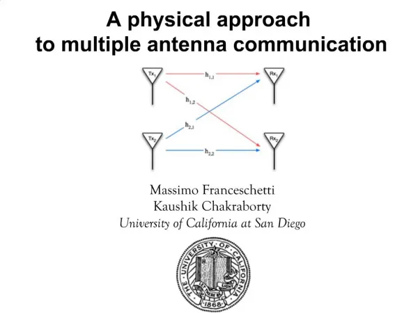
Stochastic rays propagation. MASSIMO FRANCESCHETTI University of California at Berkeley. Maxwell Equations. in complex environments. No closed form solution Use approximated numerical solvers. We need to characterize the channel. Power loss Bandwidth Correlations.

E N D
Stochastic rays propagation MASSIMO FRANCESCHETTI University of California at Berkeley
Maxwell Equations in complex environments • No closed form solution • Use approximated numerical solvers
We need to characterize the channel • Power loss • Bandwidth • Correlations
The true logic of this world is in the calculus of probabilities. James Clerk Maxwell
Simplified theoretical model solved analytically 2 parameters: hdensity gabsorption
The wandering photon Walks straight for a random length Stops with probability g Turns in a random direction with probability (1-g)
The wandering photon After a random length, with probability g stop with probability (1-g ) pick a random direction
The wandering photon r P(absorbed at r) = g(r,g,h)
Derivation pdf of hitting an obstacle at r in the first step pdf of being absorbed at r Stop first step Stop second step Stop third step
All photons entering a sphere at distance r, per unit area All photons absorbed past distance r, per unit area o o Relatingg(r,g,h)to the received power Density model Flux model
Classic approach wave propagation in random media relates comparison Validation Random walks Model with losses analytic solution Experiments
Fitting the data Power Flux Power Density
Fitting the data dashed blue line: wandering photon model red line: power law model, 4.7 exponent staircase green line: best monotone fit
The wandering photon can do more
Random walks with echoes impulse response of a urbanwireless channel Channel
Impulse response |r3| R is total path length in n steps r |r2| r is the final position after n steps o |r1| |r0|
Results Varying absorption Varying pulse width
Results Time delay and time spread evaluation Varying transmitter to receiver distance
WWW. . .edu/~massimo Papers: A random walk model of wave propagation M. Franceschetti J. Bruck and L. Shulman IEEE Transactions on Antennas and Propagation to appear in 2004 Stochastic rays pulse propagation M. Franceschetti Submitted to IEEE Trans. Ant. Prop. Download from: Or send email to: massimof@EECS.berkeley.edu