Download
1 / 56
570 likes | 595 Views
Explore N-view geometry for 3D reconstruction, epipolar geometry, fundamental matrix, feature detection, robust statistics like RANSAC, and 3D triangulation. Dive into essential matrix and calibration constraints.

E N D
ATTENTION: this is only a tentative draft, re-download it after the lectures. Two-view geometry and 3D reconstruction Why study N-view geometry? Only way to get 3d! 3 equivalent pbs.: • 3d reconstruction • motion estimation • correspondence Including traditional stereo and SFM … for calibrated setting
Intuitive epipolar geomegtry Entirely characterized by the so-called epipolar geometry Geometric notions: • epipole • epipolar lines • epipolar plane • pencil of epipolar lines and planes • baseline
u u’ O O
Algebraic characterisation of the epipolar geometry: the fundamental matrix F = [a] A
Properties of the fundamental matrix F: Note: for calibrated, it is the essential matrix (later)
x u u’ O Never neglect the coplanar case O When space points are planar, a homography relating u and u’ It is therefore a ‘collineation’ for COPLANAR points!
From P=(I 0) , P’=(A a) and a known plane p^Tx=0, to get H …
Estimation of F Given compute F • 7 pts, by linear spanning and determinant (Sturm’s algebraic method) • 8 pts, standard (and normalised) • (optimal sol.) • (robust)
8-point, standard • linear sol by svd • rank enforcement by svd!
7-point algorithm • one parameter solution by svd • from the vanishing determinant, get a cubic equation
Summary of the projective approach to 2-view geometry • F matrix • Sturm’s method of 7 pts • (8-pts algo.) More pragmatic and closer to the reality!!!
Topics on feature detection: points of interest, (or corners ) • 1D features --- edge detection --- Canny-like • 2D features --- points of interest
First derivative: The point having ||*||>threshold is a candidate, and becomes an edge point if it is a local maximum in the gradient direction. Sobel, …, Canny-like detector
Auto-correlation function: Up to first order: The point having two strong eigenvalues is a candidate, and becomes a point of interest if it is a local maximum. Harris&Stephen, Moravec-Lucas-Kanade
Matching by correlation: or Very often, on normalised images instead of I and I’
Normalisation To make the average point as close as possible to (1,1,1)! • normalisation by transformations • linear sol • rank enforcement • denormalisation
Optimal solution Rank 2 parametrisation
Robust statistics for finding correspondences From least-squares method to least median of squares (LMS) Handle ‘big errors’---outliers!
Illustrative example of fitting a line to a set of 2D points • the least squares solution (orthogonal regression) is optimal when no outliers • but it is becoming very fragile to outliers • the least median of squares is good even if 50% outliers!
LMS Repeating the following procedure: • randomly draw a sample of s data • initiate the model Mi • compute the distance to the model for each data pt • compute the median of the squares for Mi • select the Mi having the smallest value • determine inliers according to sigma (can be estimated) • re-estimate using inliers Then,
RANSAC (random sample consensus) Fischler and Bolles 1981 repeating • randomly draw a sample of s data • initiate the model Mi • compute the distance to the model for each data pt • determine inliers/outliers by the threshold t • compute the size of inliers Si • select the Mi having the largest Si • re-estimate using all inliers then
Advantage/disadvantages of RANSAC and LMS • RANSAC needs one parameter • LMS breaks down at 50%
How many times to repeat? p Probability of success (only inliers) Outlier proportion s Sample size Ex: 99.9% success rate, 50% outliers s=4, N=72 s=6, N=293 s=7, N=588 s=8, N=1177
The complete algorithm of automatic computation of F: • detect points of interest in each image • compute the correspondences using correlation based method • RANSAC or LMS using 7-pt algo. • non-linear optimal estimation on the final inliers
What can we do with F? • When calibrated, essential matrix, its decomposition • ‘motion’ estimation • Without calibration, what can we get? • Is it possible to obtain on-line calibration?
Essential matrix: fundamental matrix for the calibrated image points Relationship between E and F E = [t] R From F = [a] A Decomposition of the essential matrix into R and t The extra algebraic constraint: the equal singular values (more complicated)
Decomposition of E E = U S V^T, E=[t]R = S R then … Two factorisation Twisted pair Two translation
The five-point algorithm of the Essential matrix A long history, settled by Nister, starting from Damazure, Faugeras, Maybank, Triggs, … E = [t] R
3D reconstruction: triangulation • linear method • non-linear optimal method • compute F • given K, compute E • decompose E to get P and P’ • 3d reconstruction by triangulation
Projective reconstruction without calibration 1. This is not unique, as for any v and lambda, we have 2. Or the algebraic approach by epipolar geometry (cf. Faugeras’92 ECCV, What can be seen from an uncalibrated stereo rig?) 3. The bottome line of numerical schema is the true ‘optimal’ of F
Introduction • 3D Vision: 3D reconstruction from 2D images • Calibrated (SFM) vs. uncalibrated reconstruction • Projective reconstruction from uncalibrated images • Extra metric information to upgrade non-metric reconstruction
Self-calibration Projective metric reconstruction (uncalibrated) from only point correspondencesusing geometric self-consistency constraints The original idea of Maybank&Faugeras91 key components: absolute conic, fundamental matrix and Kruppa equation Later on: absolute quadric … Generally at least 3 images for self-calibration
1. A simple algebraic way of introducing self-calibration equation: Euclidean First ref. view Projective
2. Fundamental self-calibration equation: getting the image of the abs quadric The image of the dual absolute conic The rank 3 absolute quadric
Metric structure in projective space The absolute conic: a space conic on the plane at infinity • In point coordinates: • In plane (dual) coordinates: Rank 3 space quadric = absolute quadric
The absolute conic The plane at infinity The line at infinity of a usual plane The pair of circular points A usual plane in 3D
Metric update Eigen decompose Intrinsic difficulties: Rank constraint and semi-definite positiveness
Some common cases • Constant K: K1=K2=… • Generally quadratic equations from 3 views • Linear constraints if the principal pt is known (from zero-entries) • Constant but unknown f • Variable focal length fi (known principal pt)
A stratified approach Plane at infinity + intrinsic parameters (absolute conic) Constantness of int. param. Modulus constraint Kruppa equations If one is determined, the other is straightforward
Self-calibration using plane homographies It is possible, but not easy. Cf. Triggs ECCV98
The art of self-calibration in practice • inevitable for ‘hand-held’ camera applications (cf. 3d demo) • difficult due to ‘critical motion’ weak solution for IBR • sophisticated tools for robust solutions
x Rotating the camera around the center is equivalent to a homographical Transformation of the image plane: A pencil of lines cut by two lines A star of lines cut by two planes
2D rotating camera (for mosaicing) No translation, so no P but H: A homographic relationship H, then Hi can be also interpreted as infinite homography as u1 can be thought of the points at the plane at inf Just transformation of a conic on a plane The dual absolute conic on the plane at infinity
H can be normalized as det(H)=1 (it’s impossible for P!), then the scaling factor can be removed, so a linear system is obtained. In dual coordinates Take the inverse both sides In point coordinates