Download
1 / 30
330 likes | 592 Views
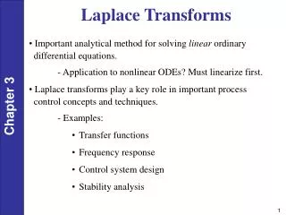
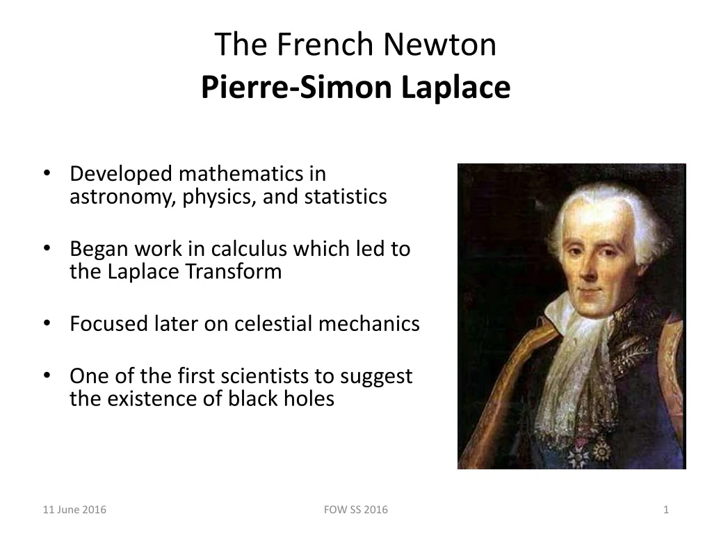
The French Newton Pierre-Simon Laplace. Developed mathematics in astronomy, physics, and statistics Began work in calculus which led to the Laplace Transform Focused later on celestial mechanics One of the first scientists to suggest the existence of black holes. Real-Life Applications.

E N D
The French NewtonPierre-Simon Laplace • Developed mathematics in astronomy, physics, and statistics • Began work in calculus which led to the Laplace Transform • Focused later on celestial mechanics • One of the first scientists to suggest the existence of black holes FOW SS 2016
Real-Life Applications Semiconductor mobility Call completion in wireless networks Vehicle vibrations on compressed rails Behavior of magnetic and electric fields above the atmosphere FOW SS 2016
Introduction FOW SS 2016
The Laplace Transform FOW SS 2016
Limitations of FT and need of LT LT can be used to analyze large class of CT problems involving signals that are not absolutely integrable. So FT based problems can not be employed in this class of problems Using LT integrodifferential equations are transformed into simple algebraic equations and convolution in time domain becomes multiplication in s domain FT is evaluated on entire jω axis ,LT is evaluated on s plane (consideration in stability) The exponential factor (Complex Number) has the effect of forcing the signals to converge, hence LT can be applied to broader class of signals
Region of Convergence (ROC) Properties of ROC: ROC Consists of strips parallel to jω axis. ROC does not contain any pole. If signal is time limited ROC is entire s plane. If signal is right sided , ROC is also right sided with σ> 0 If signal is left sided ROC is also left sided with σ< 0 A two sided signal has ROC given by a vertical strip of finite width in s plane.
Relation between LT and FT LT = FT when σ = 0 FOW SS 2016
LT of Periodic/aperiodic function FOW SS 2016
LT of Periodic/aperiodic function FOW SS 2016
LT of some standard signals FOW SS 2016
Properties of LT FOW SS 2016
LT evaluation using properties • The LT of a unit ramp function starting at t = a is ? • The LT of 3) The unilateral LT of x(t) = u(t) * tu(t) ? 4) The bilateral Laplace transform of the signal x(t) = 5) LT of x(t) = δ(at + b) ? FOW SS 2016
LT evaluation using properties 6) LT of x(t) = • LT of x(t) = • LT of x(t) = • LT of x(t) = r(2t) FOW SS 2016
Initial Value Theorem If the function f(t) and its first derivative are Laplace transformable and f(t) has the Laplace transform F(s), and the exists, then Initial Value Theorem The utility of this theorem lies in not having to take the inverse of F(s) in order to find out the initial condition in the time domain. This is particularly useful in circuits and systems. FOW SS 2016
Numerical Example: Given; Find f(0) FOW SS 2016
Final Value Theorem If the function f(t) and its first derivative are Laplace transformable and f(t) has the Laplace transform F(s), and the exists, then Final Value Theorem Again, the utility of this theorem lies in not having to take the inverse of F(s) in order to find out the final value of f(t) in the time domain. This is particularly useful in circuits and systems. FOW SS 2016
Numerical Example: Final Value Theorem: Given: . Find FOW SS 2016
Inverse Laplace Transform • L-1 s = ? • The inverse LT of X(s) = 3) The inverse LT of X(s) = FOW SS 2016
Inverse Laplace Transformation Partial fraction Expansion. “Cover up Rule” A: B: FOW SS 2016
Inverse Laplace Transformation A and B same as in previous problem. FOW SS 2016
Stability and causality in s domain FOW SS 2016
Stability and causality in s domain FOW SS 2016
Stability and causality in s domain FOW SS 2016
Laplace transforms are the primary tool used to solve DEs in control engineering. Applications of LT When initial conditions are zero: For non zero initial conditions FOW SS 2016
Transfer Function • Definition • H(s) = Y(s) / X(s) • Relates the output of a linear system (or component) to its input • Describes how a linear system responds to an impulse • All linear operations allowed • Scaling, addition, multiplication H(s) X(s) Y(s) FOW SS 2016
Example of Solution of an ODE • ODE w/initial conditions • Apply Laplace transform to each term • Solve for Y(s) • Apply partial fraction expansion • Apply inverse Laplace transform to each term FOW SS 2016
Example R L v(t) C v(t) = R I(t) + 1/C I(t) dt + L di(t)/dt V(s) = [R I(s) + 1/(C s) I(s) + s L I(s)] Note: Ignore initial conditions FOW SS 2016
Numerical on RLC circuit Step I: Apply KVL to entire circuit Step II : If initial conditions are not mentioned assume as zero. If initial conditions are given take them into account Step III : Find current i(t) from I(s) or asked parameter by taking Inverse LT FOW SS 2016
Mail id : For future communication gngaikwad.scoe@sinhgad.edu ganesh1426@gmail.com FOW SS 2016
Thank You FOW SS 2016