Exploring International Portfolio Diversification Benefits | Maximizing Returns and Minimizing Risk

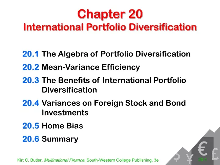
1. Chapter 20International Portfolio Diversification 20.1 The Algebra of Portfolio Diversification 20.2 Mean-Variance Efficiency 20.3 The Benefits of International Portfolio Diversification 20.4 Variances on Foreign Stock and Bond Investments 20.5 Home Bias 20.6 Summary

2. Perfect financial markets...a starting point • Frictionless markets • no government intervention or taxes • no transaction costs or other market frictions • Rational investors with equal access to costless information and market prices • All investors rationally price financial securities • All investors have equal access to costless information • All investors have equal access to market prices

3. The algebra of portfolio theory Assumptions • Nominal returns are normally distributed • Investors want more return and less risk in their functional currency xi= proportion of wealth in asset i, s.t.Si xi = 1 Expected return on a portfolio E[rP] = Si xi E[ri] Portfolio variance Var(rP) = sP2 = Si Sj xi xj sij where sij = rij si sj

4. Expected return on a portfolio E[ri] si A American 11.8% 17.8% J Japanese 15.4% 36.5% Example: Equal weights of A and J E[rP] = xA E[rA] + xJ E[rJ] = (½)(0.118)+(½)(0.154) = 0.136, or 13.6%

5. Variance of a portfolio Correlation E[ri] si A J A American 11.8% 17.8% 1.000 0.304 J Japanese 15.4% 36.5%0.304 1.000 sP2 = xA2sA2 + xJ2sJ2 + 2 xA xJ rAJ sA sJ = (½)2(0.178)2 + (½)2(0.365)2 + 2(½)(½)(0.304)(0.178)(0.365) = 0.0511 sP = (0.0511)1/2 = 0.226, or 22.6%

6. Key results of portfolio theory • The extent to which risk is reduced by portfolio diversification depends on the correlation of assets in the portfolio. • As the number of assets increases, portfolio variance becomes more dependent on the covariances (or correlations) and less dependent on variances. • The risk of an asset when held in a large portfolio depends on its covariance (or correlation) with other assets in the portfolio.

7. Diversification Mean annual return J r= -1 r = +0.304 r = +1 A Standard deviation of annual return

8. Mean-variance efficiency Mean annual return Investment opportunity set Efficient frontier J B A Standard deviation of annual return

9. The promise of internationalportfolio diversification Expected return • Potential for higher returns • Potential for lower portfolio risk W M rF Standard deviation of return

10. Domestic versus international diversification Portfolio risk relative to the risk of a single asset (sP²/si²) U.S. diversification only International diversification 1.0 0.5 26% 12% 5 10 15 20 25 Number of stocks in portfolio

11. Historical stock market performance(1970-2002)

12. International stock returns(Dollar returns to US investors from 1970-2002) Mean Stdev bWSI Canada 10.4 18.8 0.79 0.17 France 14.0 29.1 1.09 0.23 Germany 12.5 30.0 1.05 0.18 Japan 15.4 36.5 1.39 0.23 Switzerland 14.2 25.5 0.98 0.28 U.K. 14.6 29.4 1.14 0.25 U.S. 11.8 17.8 0.87 0.26 World 0.112 0.176 1.00 0.23 bW versus the MSCI world stock market index Sharpe Index (SI) = (rP- rF) / sP

13. International equity correlations(Dollar returns to US investors from 1970-2002) Can Fra Ger Jap Swi UK US France 0.472 Germany 0.388 0.645 Japan 0.320 0.399 0.364 Swiss 0.464 0.618 0.670 0.430 U.K. 0.513 0.559 0.451 0.369 0.569 U.S. 0.727 0.482 0.443 0.304 0.504 0.522 World 0.735 0.657 0.618 0.671 0.674 0.685 0.855

14. International asset allocation Foreign stocks Internationally diversified stocks and bonds U.S. stocks and bonds U.S. stocks Foreign bonds U.S. bonds “Asset Allocation.” Jorion, Journal of Portfolio Management, Summer 1989.

15. Return on a foreign asset Recall Ptd = PtfStd/f (Ptd/Pt-1d) = (1+rd) and (Std/f/St-1d/f) = (1+sd/f) Return on aforeign asset (1+rd)= (Ptd/Pt-1d) = (PtfStd/f/Pt-1fSt-1d/f) = (Ptf/Pt-1f)(Std/f/St-1d/f) = (1+rf)(1+sd/f) =1+rf+sd/f+rfsd/f (20.7)

16. Return statistics on foreign assets Expected return E[rd] = E[rf]+E[sd/f]+E[rfsd/f] Var(rd) = Var(rf)+Var(sd/f)+Var(rfsd/f) +2Cov(rf,sd/f)+2Cov(rf,rfsd/f)+2Cov(sd/f,rfsd/f) = Var(rf) + Var(sd/f) + (interaction terms)

17. Variance of return on foreign stocks(from the perspective of a US investor) Interaction Var(rf) + Var(s$/f) + terms = Var(r$) Canada 0.915 + 0.033 + 0.053 = 1.000 France 0.937 + 0.149 + -0.086 = 1.000 Germany 0.973 + 0.194 + -0.167 = 1.000 Japan 0.813 + 0.182 + 0.005 = 1.000 Switzerland 0.928 + 0.298 + -0.225 = 1.000 U.K. 0.902 + 0.127 + -0.029 = 1.000 Average 0.911 + 0.164 + -0.075 = 1.000 • The dominant risk in foreign stock markets is return variability in the local currency • Exchange rate variability is less important

18. Variance of return on foreign bonds(from the perspective of a US investor) Interaction Var(rf) + Var(s$/f) + terms = Var(r$) Canada 0.601 + 0.184 + 0.215 = 1.000 France 0.242 + 0.823 + -0.065 = 1.000 Germany 0.124 + 0.818 + 0.058 = 1.000 Japan 0.172 + 0.701 + 0.126 = 1.000 Switzerland 0.090 + 0.936 + -0.026 = 1.000 U.K. 0.287 + 0.599+ 0.114 = 1.000 Average 0.253 + 0.677 + 0.070 = 1.000 • The dominant risk in foreign bond markets is exchange rate variability • Return variability in the local currency is less important

19. Home asset bias • Despite the potential benefits of international portfolio diversification, most investors tilt their portfolios toward domestic securities.

20. The extent of home bias Portfolio weights PredictedActual Market cap as Percentage in percent of totaldomestic equities France 2.6% 64.4% Germany 3.2% 75.4% Italy 1.9% 91.0% Japan 43.7% 86.7% Spain 1.1% 94.2% Sweden 0.8% 100.0% U.K. 10.3% 78.5% U.S. 36.4% 98.0% Source: Cooper & Kaplanis, “Home Bias in Equity Portfolios, Inflation Hedging, and International Capital Market Equilibrium,” Review of Financial Studies, Spring 1994.

21. Why is there home bias?Portfolio theory can argue either way • Tilt toward more domestic assets • Domestic stock portfolios can hedge domestic inflation risk • Banks and insurance companies with domestic liabilities have an incentive to hedge with domestic assets • Tilt toward fewer domestic assets • Labor income is highly correlated with other domestic assets, so investors’ portfolios of tradable assets should be tilted away from domestic assets

22. Why is there home bias?Market imperfections • Financial market imperfections • Market frictions • Government controls • Taxes • Transactions costs • Investor irrationality • Unequal access to market prices • Unequal access to information

23. Investor irrationality • Hueristics (decision rules) • While hueristics can simplify decision-making, they also lead to cognitive biases • Frame dependence • The form in which a problem is presented can influence decisions Overconfidence should lead to higher trading volume Regret avoidance tendency to hold losers & sell winners

24. Unequal access to prices Weight in a U.S. investor’s portfolio PredictedAdjusted prediction Actual (% of cap) (% of available cap) Australia 0.24 1.30 1.25 Brazil 0.24 1.12 0.47 Canada 0.54 2.49 1.63 France 0.65 2.96 2.34 Germany 0.49 3.62 2.55 Hong Kong 0.21 1.81 1.32 Italy 0.32 1.51 1.21 Japan 1.04 9.72 7.65 Mexico 0.27 0.69 0.65 Netherlands 0.81 2.05 1.74 Sweden 0.30 1.20 1.21 Switzerland 0.47 2.53 2.39 U.K. 1.66 8.76 10.07 U.S.A. 91.29 49.60 58.32 Source: Dahlquist, Pinkowitz, Stulz, and Williamson, “Corporate Governance and the Home Bias,” Journal of Financial and Quantitative Analysis, March 2003.

25. Unequal access to information • Unequal access to information • It is difficult to get and interpret information from distant markets • Once invested, it is difficult to monitor the actions of distant managers • Empirical evidence • Individuals prefer investments that are culturally similar and geographically nearby

26. Appendix 20-AContinuous compounding and emerging market returns rt= ln(1+rt) = ln(Pt/Pt-1) = ln(Pt)-ln(Pt-1) r0,T = ln[ (1+r1) (1+r2)…(1+rT) ] = ln(1+r1) + ln(1+r2) + … + ln(1+rT)] = [r1+r2+…+rT] = ln(PT/P0) ravg = [r1+r2+…+rT]/T Continuously compounded returns are additive over time

27. Continuously compounded returns are symmetric r1=100% 200 r1=+69.3% r2=-69.3% 100 100 r2=-50% ravg = ln[(1+r1)(1+r2)]/2 = ln[(1+r1)+ln(1+r2)]/2 = (r1+r2)/2 = (+0.693-0.693)/2 = 0

28. Emerging markets:Holding period returns • The normal distribution is not a good fit to holding period return distributions • Based on monthly returns to the MSCI emerging market indices over 1988-2002 • 20 of 26 have positive skewness • 25 of 26 have excess kurtosis relative to the normal distribution

29. Emerging markets:Continuously compounded returns • The normal distribution is a better fit to continuously compounded returns • Based on monthly returns to the MSCI emerging market indices over 1988-2002 • 10 of 26 have positive skewness • 25 of 26 have excess kurtosis relative to the normal distribution There remains evidence of leptokurtosis (a few extreme returns in each tail)

30. Returns to MSCI’s S. Korea index Linear scale

31. Returns to MSCI’s S. Korea index Logarithmic scale

32. Monthly returns are positively skewed and fat-tailed The MSCI Korea index(Jan 1988 - Jan 2003)

33. Continuously compounded returns are fat-tailed, but fairly symmetric The MSCI Korea index(Jan 1988 - Jan 2003)

34. RiskMetrics conditional volatility st2 = (0.97)st-12 + (0.03)st-12 Korea

35. Holding period returns(annual returns in U.S. dollars)

36. Continuously compounded returns(annual returns in U.S. dollars)

37. Correlations, betas, and risks • Periodic compounding exaggerates the arithmetic means and standard deviations • The compounding method has much less of an effect on correlations and betas The Korean market provides an example • With holding period returns m = 16.3%, s = 58%, rK,W = 0.424, bK = 1.214 • With continuous compounding m = 2.8%, s = 53%, rK,W = 0.434, bK = 1.183