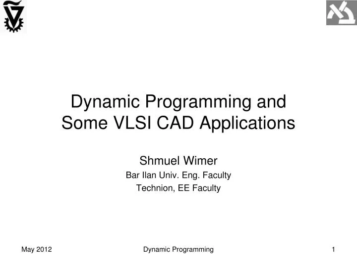
Dynamic Programming and Some VLSI CAD Applications

1. Dynamic Programming andSome VLSI CAD Applications Shmuel Wimer Bar Ilan Univ. Eng. Faculty Technion, EE Faculty Dynamic Programming

2. Outline • NP Completeness paradox • Efficient matrix multiplication by dynamic programming • Dynamic programming in a tree model • Optimal tree covering in technology mapping • Optimal floor planning • Optimal buffer insertion • Dynamic programming as sequential decision problem • Resource allocation • The knapsack problem • Automatic cell layout generation • Optimal wire sizing Dynamic Programming

3. NP Completeness Paradox Dynamic Programming

4. Dynamic Programming

5. Dynamic Programming

6. Dynamic Programming

7. Optimal Matrix-Chain Multiplication Dynamic Programming

8. Dynamic Programming

9. Dynamic Programming

10. Dynamic Programming

11. Dynamic Programming

12. Dynamic Programming

13. Dynamic Programming

14. 2 2 3 3 4 4 5 5 6 6 i=1 i=1 J=6 J=6 5 5 4 4 3 3 2 2 1 1 m[1..6,1..6] s[1..6,1..6] Dynamic Programming

15. Dynamic Programming

16. Dynamic Programming

17. Elements of Dynamic Programming • A problem exhibits optimal substructure if an optimal solution to the problem contains within it optimal solutions to sub problems. • In a sequence of decisions the remaining ones must constitute optimal solutions regardless of past decisions. (principle of optimality). • The space of sub problems must be small, namely, a recursive solution must solve same problem many times. Optimization problem has overlapping sub-problems. Dynamic Programming

18. Overlapping sub-problems called by recursive solution are memorized (encoded in a table), hence addressing their solution only once. • Optimal solution is constructed by backtracking. Dynamic Programming

19. Optimal Tree Covering A problem occurring in mapping logic circuit into new cell library. Given: • Rooted binary tree T(V,E) called subject tree (cone of logic circuit), whose leaves are inputs, root is an output and internal nodes are logic gates with their I/O pins. • A family of rooted pattern trees (logic cells of library), each associated with a non-negative cost (area, power, delay). Root is cell’s output and leaves are its inputs. Dynamic Programming

20. A cover of the subject tree is a partitioning where every part is matching an element of library and every edge of the subject tree is covered exactly once. Find a cover of subject tree whose total sum of costs is minimal. Dynamic Programming

21. t4 (4) t1 (2) t2 (3) t3 (3) t5 (5) r s t 4+2+3=9 3+5=8 3+2+2+3=10 t3 t5 u t3 t1 t4 t1 t1 t2 t2 Dynamic Programming

22. INV (1) a NAND2 (2) c NAND2 (2) b e INV (1) f d j NAND3 (3) INV (1) g NAND2 (2) h i AOI21 (3) NAND2 (5) NAND2 (8) INV (9) AOI21(6) NAND2 (11) NAND3 (12) INV (3) NAND2 (5) NAND3 (3) Observation: pattern p rooted at the root of T(V,E) yields minimal cost only if the cost at any of p’s leaves is minimal, suggesting bottom-up matching algorithm. Dynamic Programming

23. Dynamic Programming

24. v ? ? ? ? ? ? ? u , q u , q Optimal Buffer Insertion Dynamic Programming

25. R4 4 C4 R2 2 R5 5 C3 R1 0 C5 1 R6 C1 6 R3 C6 3 C2 R7 7 C7 Delay Model Dynamic Programming

26. sub-tree RM (TM , LM) M (T’K , L’K) CM RK K sub-tree CK RN N (TN , LN) CN Bottom-Up Solution (TK , LK) Dynamic Programming

27. LN LM L’K TN TM T’K Outline of Algorithm With b nodes, 2b buffer insertions exist. There’s a polynomial solution! Merging sub-tree solutions at a parent node takes linear time! + = Dynamic Programming

28. driver’s resistance receiver’s load line-to-line coupling line resistance line-to-line coupling signal's activity, 0<=AF <=1 Interconnect Signal Model Using Elmore delay model, simple, inaccurate but with high fidelity Dynamic Programming

29. σ1 Si σi Ci Wi Ri Si+1 A L σn-1 σn Interconnect Bus Model Dynamic Programming

30. Delay and Dynamic Power Minimization signal’s delay: signal’s dynamic power: Dynamic Programming

31. Minimize bus delay Minimize bus power Subject to: In 32nm node and beyond spaces and widths are very few discrete values Continuous optimization and its well-known results are invalid. The sizing problem is NP-complete. A pseudo polynomial resource allocation dynamic programming solution is suitable. Dynamic Programming

32. Dynamic Programming

33. Dynamic Programming

34. Floorplan Floorplan and Layout Graph representation B1 B2 B7 B8 B8 B2 B7 B9 B1 B9 B12 B10 B5 B10 B3 B3 B5 B4 B12 B11 B6 B11 B6 B4 Floorplan is represented by a planar graph. Vertices - vertical lines.Arcs - rectangular areas where blocks are embedded. A dual graph is implied. Dynamic Programming

35. From Floorplan to Layout • Actual layout is obtained by embedding real blocks into floorplan cells. • Blocks’ adjacency relations are maintained • Blocks are not perfectly matched, thus white area (waste) results • Layout width and height are obtained by assigning blocks’ dimensions to corresponding arcs. • Width and height are derived from longest paths • Different block sizes yield different layout area, even if block sizes are area invariant. Dynamic Programming

36. v h h v v v v h h h h B7 B12 B1 B2 B3 B5 B8 B10 B4 B6 B9 B11 Optimal Slicing Floorplan Top block’s area is divided by vertical and horizontal cut-lines Slicing tree. Leaf blocks are associated with areas. B1 B2 B7 B8 B9 B12 B10 B3 B5 B11 B6 B4 Dynamic Programming

37. Dynamic Programming

38. v + = + = + = Merge horizontally two width-height sets (vertical cut-line) Dynamic Programming

39. h Size of new width-height list equals sum of lengths of children lists, rather than their product. Dynamic Programming

40. Sketch of Proof • Problem is solved by a bottom-up dynamic programming algorithm working on corresponding slicing tree. • Each node maintains a set of width-height pairs, none of which can be ruled out until root of tree is reached. Size of sets is in the order of node’s leaf count. Sets in leaves are just Bi’s two orientations. • The sets of width-height pairs at each node is created by merging the sets of left-son and right-son sub-trees in time linear in their size. • Width-height pair sets are maintained as a sorted list in one dimension (hence sorted inversely in the other dimension). • Final implementation is obtained by backtracking from the root. Dynamic Programming

41. Cost=0 Cost=1 Cost=2 Vcc Vcc a a Vcc Vcc Vcc a a a a a Vcc Vcc Vss Vss b b b Vss b b Vss Vss Vss Vss b b Automatic Cell Layout Generation • 3 step process: • Transistor placement • Interconnect completion • Design rule adherence • Transistor placement comprises: • Transistor P-N pairing • Pair ordering • Pair flipping – optimize cell area, node cap, potential cell abutment, cell’s internal routing Dynamic Programming

42. Most cells unfortunately contain more than 4 transistors. • A flip configuration of a pair depends on the flip of its left and right neighbors. • Seek the flip configuration yielding minimal sum of abutment cost. • With n pairs, there are 2n solutions to consider. • Observation: An optimal flip of j+1 pairs subject to given right end configuration of pair j necessitates that the first j pairs have been optimally flipped. • Principle of optimality, optimal sub problem solutions. • Observation: The optimal flip of rest n – j pairs is independent of the first j flips except the right end configuration of pair j. • This defines a state for which only the lowest cost flip of j pairs is of interest. • Dynamic Programming solution is in order. (Bar-Yehuda et. al.) Dynamic Programming

43. stage j a a c c abutment cost b b d d a a c c d d b b a a c c d d b b c c a a b b d d State Augmentation stage j+1 Dynamic Programming

44. Dynamic programming takes O(n) time. • Can be extended to multi-row cell (double height, etc.). • It can be combined in a DFS algorithm which considers simultaneously paring, pair ordering and optimal flip, without any complexity overhead (state augmentation takes O(1) time) • Dynamic programming is solving in fact a shortest path algorithm on the state transition graph. • New litho rules in 32nm and smaller feature size offer many optimization opportunities. Dynamic Programming

45. Resource Allocation Dynamic Programming

46. Dynamic Programming

47. Elements of Dynamic Programming • Sequential decision making process. • Transition occurs from state to state. • A state is a summary of prior history of the process sufficiently detailed to enable evolution of current alternatives. • Sequential decision process evolves from state to state. • The pair (j,y) is a state in the resource allocation process. • The elements encoded in a state are called state variables. • Principle of optimality states that whatever the initial state is and decisions were, the remaining decisions must constitute an optimal policy. Dynamic Programming

48. Linear Case: Knapsack Problem Dynamic Programming

49. Linear Case: Knapsack Problem Dynamic Programming