Download
1 / 20
200 likes | 317 Views
Linear Optics Corrections. RHIC: Todd Satogata, Mei Bai, Jen Niedziela AGS: Vincent Schoefer, Kevin Brown, Leif Ahrens, … November 3, 2006. Objective Reduce machine/model difference in optics, in both directions! Orbit Response Matrix AC Dipole Optics AGS Orbit Response Matrix.

E N D
Linear Optics Corrections RHIC: Todd Satogata, Mei Bai, Jen Niedziela AGS: Vincent Schoefer, Kevin Brown, Leif Ahrens, … November 3, 2006 • Objective Reduce machine/model difference in optics, in both directions! • Orbit Response Matrix • AC Dipole Optics • AGS Orbit Response Matrix
Response Matrix Background • Originally used by Corbett, Lee, and Ziemann at SPEAR, 1993 • Popularized by Safranek at NSLS X-Ray Ring, 1994-6 • Orbit response matrix (with coupling/nonlinear feeddown): where (x,y) are corrector setting changes and (x,y) are measured difference orbits from these corrector settings. (There are also dispersive terms in Rij when fRF=constant, as was the case in RHIC measurements.) • Compare model and measured R “response matrices”, and iteratively make model changes to converge to agreement. • “Model changes” include quad gradients, BPM/corr gains, … • Measures gradient errors, BPM/corr gain errors, skew errors, … • RHIC AT storage lattices include snake matrices from Waldo T. Satogata - APEX Linear Optics
Response Matrix Background • The difference between Rmodel and Rmeasured is written as a single vector with length (NbpmsxNcorrs), and expanded in terms of variable changes vk, that include quad gradient errors, corrector and BPM gain errors, skew errors, etc: • This can be solved for vk with SVD, assuming a good model for . The quadrupole gradient error dependence is nonlinear, so the SVD solution is iterated through the model until it converges. Weight with BPM noise I T. Satogata - APEX Linear Optics
Simulation Results: No BPM Noise • Tested yellow store lattice, random –0.1 to 0.1% quad errs • With no BPM noise, fitting is “perfect” • Lattice is therefore nondegenerate T. Satogata - APEX Linear Optics
Issue: BPM Noise from 10 Hz • Average orbit noise at store: 30-40 um horizontal peak-peak • 7800 turn averaging gives 15-20 um peak-peak • Need ~10 orbits per data point to achieve 5 um BPM noise, including BPM change to average orbit sampling period T. Satogata - APEX Linear Optics
0.2% beta beat after fit 20% beta beat before fit Simulation Results: 30 um BPM Noise • With 30 um BPM noise, error bars are larger than errors • Fits are inexact, but method still converges – not unique • Beta beating is reduced by two orders of magnitude T. Satogata - APEX Linear Optics
Before After BPM error vs fit Corrector error vs fit Simulation Results: 30um BPM Noise and BPM/Corrector Gains • Simulation fits of BPM/corrector gains, 30 um BPM noise • Fits are very good, reduce gain errors by factor of 20 • BPM/gain errors and optics can be fit with 30 um BPM noise T. Satogata - APEX Linear Optics
APEX Data Acquisition and ORM Data Summary (pp35) • Data acquisition and analysis: • Takes 1-2 hours for all correctors in either RHIC ring • Both rings done in parallel for storage measurement • 3 average orbits acquired for each corrector setting • Need to automate analysis, tedious BPM/corrector alignment and orbit averaging • Measure/monitor tunes throughout measurement • No good blue injection ORM data acquired during Run-6 • Yellow injection data taken during blue polarimeter pumpdown T. Satogata - APEX Linear Optics
30-50% “signal”, chi^2=54 ORM reduces difference, chi^2 by >10 Beam Experiment Analysis: pp35 Yellow Store Q1/8/9 • Use only arc BPMs, fit Q1/Q8/Q9 quadrupoles • Appears to converge, chi^2 reduces by factor 10 • Beta beating is 10-15% horizontal, over 40% vertical! • Fitted quadrupole errors are still too large by at least x10 • Example: yi6-qf8 fit converges to a change of –5% ! Check data T. Satogata - APEX Linear Optics
ORM reduces difference, chi^2 by 20 Beam Experiment Analysis: pp35 Yellow Store Q1/4-9 • Use only arc BPMs, but now fit Q1/4-9 quadrupoles • Appears to converge better, chi^2 reduces by factor 20 • Beta beating is consistent with previous result, smoother • Fitted quadrupole errors are even larger, up to 8%! • Need to double-check data; these errors are unphysical T. Satogata - APEX Linear Optics
Yi6-qf1 Measured Yellow Store AC Dipole Beta Beat • Measured beta beat in the Yellow ring at store energy: fit is only yi6-qf1 has a 10% KL error! • The gradient error is obtained by . Here R can be calculated from the model • plan: • to finish the data analysis: Yellow injection and Blue at store and injection • dedicated gradient error measurement at injection Not consistent with ORM data! M. Bai T. Satogata - APEX Linear Optics
Future Plans • Careful analysis of existing data • Remove suspicious data, hand-match full ORM matrices • Aggressive singular value cuts; existing too permissive? • Blind baseline APEX • Insert and measure known quadrupole errors • Improve BPMs, reduce data acquisition noise • Change BPM average orbit sampling time • Increase number of orbits acquired per corrector setting • Reduce dimensionality • Typically 20-25% of correctors are used (FNAL, ALS) • Speeds up data acquisition, analysis, reduces memory requirements • Coupling analysis • Reduced dimensionality should allow this T. Satogata - APEX Linear Optics
APEX Requests and Requirements • 2-3h Blue testing at injection during startup period • Decouple; separate/measure tunes for lattice fit; save model • Measure dispersion before and after ORM measurement • BPMs averaging set to 7800 turns to limit 10 Hz (nth turn?) • Measure BPM average orbit noise at all BPMs • Compare difference orbit measurement/prediction, dispersion • Measure ORM/correct optics/recheck if differences above noise • AC dipole and ORM optics measurements • Fit all quads to improve model, IR knobs to improve machine • (Fast) blind baseline measurement for AC dipole analysis • Remeasure after analysis and correction for validation • 3h Storage optics measurement/correction • Repeat above setup, including BPM noise baseline • 6 bunches, uncogged, acquire both rings simultaneously • AC dipole measurement immediately after ORM measurement T. Satogata - APEX Linear Optics
AGS ORM Measurement Data • At extraction, near integer resonance, June 15 2006 • 2-3mm response, need to filter out some bad data V. Schoefer T. Satogata - APEX Linear Optics
AGS MAD-X and Matlab/AT Comparison T. Satogata - APEX Linear Optics
AGS Simulated Error ORM Fit • Simulated/matched 5% errors in a03, c17, e03, j17 quads • All four simulated errors fit to high precision • To Do: Noise analysis, filter input data for LOCO analysis T. Satogata - APEX Linear Optics
Conclusions • RHIC ORM Simulations • RHIC storage lattice looks nondegenerate (even triplets) • BPM/corrector gains, 0.1% gradient errors, and beta beating correction can be found with realistic BPM noise (30um) • RHIC ORM Data Analysis and APEX • Present analysis doubtful, converges to large (10%) errors • Hand-correlate data to triple-check for oversights • Reduce BPM average orbit noise (sampling, more data/point) • Parasitic setup/testing with Blue beam at injection • 3h for ramping/store gradient error measurement/correction • RHIC AC Dipole APEX • Parasitic (e.g. after) above ORM APEX, complementary • AGS ORM • Studying extraction lattice, matches MAD-X • Evaluating susceptibility to BPM noise • Have ORM data in hand for analysis T. Satogata - APEX Linear Optics
========================== T. Satogata - APEX Linear Optics
Twiss Parameter Measurements • Hoffstaetter, Keil, and Xiao (EPAC 2002) • Iteratively fit cos/sin variations of (1) to measured Rij • Alternate between corrector and BPM (,) fitting • Least-squares is solved with SVD of: T. Satogata - APEX Linear Optics
Response Matrix Dimensions at RHIC • Each RHIC ring has • 334 BPM measurements (167 per plane) • 234 correctors (117 per plane) • Total response matrix size is 78156 points • APS/FNAL use only 25-40 correctors, all BPMs (Sajeev) • Fitting parameters • 334 BPM measurement gains (offsets subtract out) • 232 corrector strength gains (assume two are perfect) • 117 path length changes for horizontal correctors • 246 main/IR quadrupole gradients (or 72 IRs) • (144 chromatic sextupole offsets) • Total fitting parameters: 929 (more or less) • Total size of fit matrix: 78156*929 = 70 Mpoints • Grows larger very quickly with additional fit parameters • Minimize dimensionality to improve speed T. Satogata - APEX Linear Optics