Download
1 / 19
190 likes | 203 Views
Explore integrating build-up and interaction phases of electron cloud simulations using boosted frame methods for beam dynamics research. Benchmarking codes and planning future simulations.

E N D
Boosted frame e-cloud simulations J.-L. Vay Lawrence Berkeley National Laboratory SciDAC-II Compass Compass 2009 all hands meeting - Beam Dynamics session Tech-X, Boulder, CO - Oct 5-6, 2009
Toward fully self-consistent e-cloud simulations • To date, electron cloud distributions have been predicted using ‘build-up’ simulations (using Posinst, Ecloud, Cloudland, Warp,…) and provided as inputs to codes calculating their interaction with the beam. build-up • This mode of operation is dictated by the widely separate time scales associated with the beam and electrons dynamics: the quasistatic or the boosted frame* methods are used to bridge the time scales in codes like Headtail, QuickPIC, Pehts, CMAD, Warp,…. electron streamlines beam quasistatic boosted frame *J.-L. Vay, Phys. Rev. Lett.98, 130405 (2007)
Toward fully self-consistent e-cloud simulations • This model is appropriate for single bunch instability but fails to capture memory effects for multibunch instabilities. • Toward integrating the build-up and interaction phases, we have modified routines related to electron build-up in Warp to accommodate calculations in a boosted frame: • calculation of velocity and angle of particles impacting surfaces, • generation of secondary electrons, • background gas ionization. bunch n+1 bunch n
Modified routines successfully benchmarked on SPS toy problem • The build-up of electrons was simulated in a fully self-consistent simulation in a boosted frame (=27). • Electrons generated from gas ionization and secondary emission at walls. • Assumed continuous focusing. • One bunch was simulated, the bunch train being emulated by periodic BC. • Excellent agreement with simulations: • in the laboratory frame, • from the LBNL build-up code Posinst (M. Furman), • Warp running in build-up mode.
Fully self-consistent simulation of e-cloud driven instability • The background gas pressure was x10, to trigger a strong instability. • At these high electron densities, the electron space charge is large, which may explains observed differences between build-up and full 3D calculations. This is under investigation. If not properly resolving the betatron frequency, the choice of the parameter = time step/betatron frequency is critical.
Plans • Implement calls to gas ionization and secondary electrons generation in Warp’s quasistatic class, • Compare fully self-consistent (build-up+beam tracking) simulations between full PIC in a Lorentz boosted frame and quasistatic, cross-benchmarking and assessing the pros and cons of each approach. • Replace continuous focusing by FODO lattice and redo above. • Modify photo-electron generation class to accommodate boosted frame calculations. • Add Monte-Carlo generation of photons radiated by beam, and the generation of photo-electrons at wall. • Pursue benchmarking with other ecloud codes (to complement extensive benchmarking done with Headtail and Posinst to date).
Benchmarking of Warp vs Headtail-1 No dipole field • LHC • =479.6 • Np=1.11011 • continuous focusing • x,y=66.0,71.54 • x,y=64.28,59.31 • longitudinal motion OFF • ne=1012-1014 • Nb ecloud station/turn=10-100 • dipole magnetic field effect: frozen x-motion of electrons • same initial distribution of macro-protons with initial offset of 0.1y e- motion frozen in x
Benchmarking of Warp vs Headtail-2 • LHC • =479.6 • Np=1.11011 • continuous focusing • x,y=66.0,71.54 • x,y=64.28,59.31 • longitudinal motion ON • ne=1012-1014 • Nb ecloud station/turn=10-100 • No dipole magnetic • same initial distribution of macro-protons with initial offset of 0.1y
Benchmarking of Warp vs Headtail-3 ne=1012m-3 ne=1014m-3 • LHC • =479.6 • Np=1.11011 • continuous focusing • x,y = 66.0, 71.54 • x,y,z = 64.28, 59.31, 0.0059 • = 3.4710-4 • p/p = 4.6810-4 • chromx,y = 2., 2. • ne=1011-1014 • Nb ecloud station/turn=10-100 • dipole magnetic field effect: frozen x-motion of electrons • same initial distribution of macro-protons with initial offset of 0.1y • threshold 2-particle model for TMCI ne=1013m-3 ne=1011m-3 ne=1012m-3 ne=1014m-3 ne=1013m-3 ne=1011m-3 ≈ 6.431011
E-cloud: benchmarking against quasistatic model for LHC scenario The “quasistatic” approximation uses the separation of time scales for pushing beam and e-cloud macro-particles with different “time steps”: used in QuickPIC (USC/UCLA), Headtail (CERN), PEHTS (KEK), CMAD (SLAC), Warp (LBNL), … Excellent agreement on emittance growth between boosted frame full PIC and “quasistatic” for e-cloud driven transverse instability in continuous focusing model of LHC: The 2 runs have similar computational cost, thus how to choose one method other another? • boosted frame method offers less approximation to the physics, which may matter in some cases, • parallelization of quasistatic codes more complicated due to pipelining in the longitudinal direction.
Other possible complication: inputs/outputs • Often, initial conditions known and output desired in laboratory frame • relativity of simultaneity => inject/collect at plane(s) to direction of boost. • Injection through a moving plane in boosted frame (fix in lab frame) • fields include frozen particles, • same for laser in EM calculations. • Diagnostics: collect data at a collection of planes • fixed in lab fr., moving in boosted fr., • interpolation in space and/or time, • already done routinely with Warp for comparison with experimental data, often known at given stations in lab. frozen active z’,t’=LT(z,t)
x/t= (L/l, T/t)* FB-rest frame of “B” 0 y y 0 x x 0 space+time 0 0 • is not invariant under the Lorentz transformation: x/t . • There exists an “optimum” frame which minimizes it. • Result is general and applies to light beams too. *J.-L. Vay, Phys. Rev. Lett.98, 130405 (2007) Range of space and time scales spanned by two identical beams crossing each other F0-center of mass frame space
frame ≈ 19 3cm Hendrik Lorentz 1.6mm 1m 30m compaction x560 1.6mm/30m=53. 3cm/1m=30,000. frame ≈ 22 frame ≈ 4000 2.5mm 450m 10km 10m 1nm 4m 1nm 4.5m 10cm compaction x103 compaction x3.107 10km/10cm=100,000. 450m/4.5m=100. 2.5mm/4m=625. 10m/1nm=10,000,000,000. Lorentz transformation => large level of compaction of scales range Laser-plasma acceleration boosted frame Free electron lasers HEP accelerators (e-cloud)
Consequence for computer simulations # of computational steps grows with the fullrange of space and time scales involved Choosing optimum frame of reference to minimize range can lead to dramatic speed-up for relativistic matter-matter or light-matter interactions. electron streamlines • Calculation of e-cloud induced instability of a proton bunch* • Proton energy:g=500 in Lab • L=5 km, continuous focusing Code: Warp (Particle-In-Cell) beam (from Warp movie) proton bunch radius vs. z CPU time (2 quad-core procs): • lab frame: >2 weeks • frame with2=512: <30 min Speedup x1000 *J.-L. Vay, Phys. Rev. Lett.98, 130405 (2007)
n+1Vn+1 + nVn qt m 2 n+1/2 Vn+1 + Vn qt m 2 (with , , , , , , ). Seems simple but ! . Algorithms which work in one frame may break in another. Example: the Boris particle pusher. • Boris pusher ubiquitous • In first attempt of e-cloud calculation using the Boris pusher, the beam was lost in a few betatron periods! • Position push: Xn+1/2 = Xn-1/2 + Vn t -- no issue • Velocity push: n+1Vn+1 = nVn + (En+1/2 + Bn+1/2) issue: E+vB=0 implies E=B=0=> large errors when E+vB0 (e.g. relativistic beams). • Solution • Velocity push: n+1Vn+1 = nVn + (En+1/2 + Bn+1/2) • Not used before because of implicitness. We solved it analytically* *J.-L. Vay, Phys. Plasmas15, 056701 (2008)
Simulations of e-cloud instability in SPScomparison Warp-Headtail Eb=26 GeV (at injection) Eb=120 GeV • SPS • Np=1.11011 • ne=1.1012m-3 (uniform) • :continuous focusing • x,y= 33.85, 71.87 • x,y= 26.13, 26.185 • chrom.x,y=0.1,0.1 • // : z= 0.00323 • Warp/HT (isyn=1): continuous focusing • HT (isyn=4): focusing more localized • 10 stations/turns • 512 turns Good agreement between Warp and Headtail on emittance growth and tune shift using continuous focusing models at 26GeV and 120GeV. ec feedback simulations - JL Vay, et al.
Simulations of e-cloud instability in SPScloser look at tune shift Eb=26 GeV Eb=120 GeV tail head tail head Warp Headtail (isyn=1) Headtail (isyn=4) ec feedback simulations - JL Vay, et al.
Simulations of e-cloud instability in SPSat injection - higher electron density • SPS at injection (Eb=26 GeV) • Np=1.11011 • ne=31012m-3 (uniform) • continuous focusing • x,y= 33.85, 71.87 • x,y= 26.12, 26.185 • chrom.x,y=0.,0. • z= 0.0059 Fractional emittance growth horizontal vertical tail head Warp tail head Headtail ec feedback simulations - JL Vay, et al.