GLOBAL MOTION ESTIMATION OF SEA ICE USING SYNTHETIC APERTURE RADAR IMAGERY

1. GLOBAL MOTION ESTIMATION OF SEA ICE USING SYNTHETIC APERTURE RADAR IMAGERY Mani V. Thomas

2. Problem Statement • Sea-Ice dynamics is composed of • Large global translation • Small local non-rigid dynamics • Robust estimation of global motion provides a base for processing of non-rigid components • “Given a pair of ERS – 1 SAR images, this thesis presents a method of estimating the global motion occurring between the pair robustly”

3. Introduction • Investigation into the robust estimation of the global motion of sea ice as captured by the European Remote Sensing Satellite (ERS) imagery. • Reasons for estimation complexity • Differences in the swaths of the satellite and the rotation of the earth • the local sea-ice dynamics is over shadowed by the large magnitudes of the global translation • Time difference between the adjacent frames (typically three days due to polar orbit constraints) • Influence of fast moving storms • Significant non-linear changes in the discontinuities occur at temporal scales much lesser than 3 days

4. Motion Estimation Problem • “Optic Flow is computed as an approximation of the image motion defined as the projection of the velocities of 3-D surface points onto the imaging plane” [Beauchemin, 1995] • Image Brightness Constancy assumption • Apparent brightness of a moving object remains constant [Horn, 1986] • Under the assumption of extremely small temporal resolution the optic flow equation is considered valid

5. Motion Estimation Problem • Estimation techniques can be classified into three main categories [Kruger, 1996] • Differential methods [Horn, 1981] [Robbins, 1983] • Image intensity is assumed to be an analytical function in the spatio-temporal domain • Iteratively calculates the displacement using the gradient functional of the image • work well for sub-pixel shifts but they fail for large motions • extremely noise sensitive due numerical differentiation • convergence in these methods can be extremely slow

6. Motion Estimation Problem • Area based methods [Jain, 1981], [Cheung, 1998] • The simplest way in terms of both hardware and software complexity • Implemented in most present day video compression algorithms [ISO/IEC 14496-2, 1998; ITU-T/SG15, 1995] • Estimation is performed by minimizing an error criterion such as “Sum of Squared Difference” • Not satisfied completely since motion in real life can be considered a collage of various types of motions

7. Motion Estimation Problem • Feature based methods • Identify particular features in the scene • computes the “feature points” between the two images using corner detectors [Harris, 1998; Tomasi, 1991] • Deducing the motion parameters by matching the extracted features • Matching the detected feature between the two images using robust schemes such as RANSAC [Fischler, 1981] • Full optic flow is known at every measurement position • Only a sparse set of measurements is available • Reduction of the amount of information being processed

8. Fourier Theory • Fourier Transform of Aperiodic signals • Fourier Analysis equation • Fourier Synthesis equation • Fast Fourier Transform [Cooley, 1965] • Reduces computation from to • Fourier shift Theorem • Delay in the time domain of the signal equivalent to a rotation of phase in the Fourier domain

9. Fourier Theory • Phase Correlation • Given cross correlation equation in Fourier Domain • Inverse Fourier Transform of the product of the individual forward Fourier Transforms • By the Fourier Shift Theorem in 2D • Sharpening the cross correlation using and [Manduchi, 1993] • Inverse Fourier Transform provide a Dirac delta function centered at the translation parameters

10. Global Motion Estimation • Generalized Aperture Problem • Uncertainty principle in image analysis • Smaller the analysis window, greater the number of possible candidate estimates • Larger the analysis window size, the greater is the probability that the analysis window has a combination of various motions • Handle the motion estimation at multiple resolutions • Information percolation from coarser resolution to finer resolution in a computationally efficient fashion. • Motion smaller than the degree of decimation is lost

11. Global Motion Estimation • Global translations, in ERS-1images, are on the order of 100 to 200 pixels • “Normalized Cross Correlation” (NCC) or “Sum of Squared Distance” (SSD) require large support windows to capture the large translation • Large support windows encompass a combination of various motions • Images have varying degrees of illumination due to the degree of back scatter • SSD is extremely sensitive to the illumination variation though computationally tractable • NCC is invariant to illumination but is computationally ineffective

12. Global Motion Estimation • Phase correlation is illumination invariant [Thomas, 1987] • Characterized by their insensitivity to correlated and frequency-dependent noise • Calculations can be performed with much lower computational complexity with 2-D FFT • It can be used robustly to estimate the large motions [Vernon 2001] [Reddy, 1996] [Lucchese, 2001] • Separation of affine parameters from the translation components [De Castro 1987] [Lucchese 2001] [Reddy 1996] • Main disadvantage is applicability only under well-defined transformations

13. Global Motion Estimation • Phase Correlation v/s NCC • Uni-modal Motion distribution within the search window • Phase correlation and NCC have maxima at the same position • Multi modal motion distribution within search window • NCC produces a number of local maxima • Phase correlation produces reduced number of possible candidates Remark: Basis for support in both methods have been maintained at 96 pixels window

14. Global Motion Estimation • Histogram Equalization by Mid-Tone modification • Image enhancement and histogram equalization performed over “visually significant regions” as against the entire image • Simple histogram equalization suffers from speckle noise and false contouring [Bhukhanwala, 1994] • Experiments indicate that estimated motion field had the smallest error variance under mid tone modification

15. Global Motion Estimation • Creation of Image Hierarchy by Median Filtering • Multi-resolution image hierarchy by decimation in the spatial scale [Burt, 1983] • Aliasing due to the signal decimation • Reduced using Median filtering • Small motions tend to get masked during the process of image decimation • Masking is advantageous for global motion estimation • Motion Estimation in Image Hierarchy • Motion estimated at the coarsest level of the pyramid • Estimate is percolated to the finer levels in the pyramid by warping the images towards one another • Process iterated until the finest level of the pyramid • Reduces the computational burden since the coarse estimate is performed on smaller images

16. Global Motion Estimation • Histogram based global motion Estimation • Images divided into a tessellation of blocks, each block centered within a predefined window. • Window size, Block size and pyramid levels obtained as a parameter from the end user • Motion estimated at each block using phase correlation • Potential candidates are selected such that their magnitudes are higher than a threshold • The best possible estimate obtained from the potential candidates using the “Lorentzian estimator” [Black, 1992] • The global motion at a level of pyramid is obtained as the mode of the motion vectors at that level

17. Global Motion Estimation • Due to the periodic nature of the Discrete Fourier Transform, the maximum measurable estimate using the Fourier Transform of a signal within a window of size W is W/2. • To capture translations of magnitude (u, v), the W should be >= 2*max(u,v) • For the ERS-1 experimentation, the block size was taken as 32X32 and the window size was taken as 128X128. • The sizes of the window and the block are maintained a constant throughout the entire pyramid hierarchy • Amplification of the estimates at the finer level of the pyramid

18. Functional Description of Modules • The first level image processing related functional units. • The image reader reads the image into buffers • The image modifier that performs histogram equalization • Create image hierarchy • The second level performs the global motion estimation • Performs phase correlation on the image pyramid • analyzer functional module performs histogram analysis of the motion data • The final level performs local motion estimation • Affine components of the local non rigid deformations or a higher order parametric model

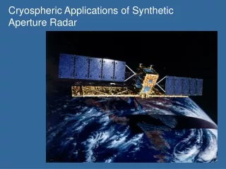
19. Data Sets • The European Space Agency’s ERS – 1 and ERS – 2 C-band (5.3 GHz) Active Microwave Instrument generate RADAR images of the Southern Ocean sea-ice cover in Antarctica, in particular the Weddell Sea • Weather independent (day or night) • Frequent repeat • High resolution 100 km swath • The 5 month Ice Station Weddell (ISW) 1992 was the only winter field experiment performed on the Western Weddell Sea. • The orbit phasing of the ERS – 1 was fixed in the 3-day exact repeating orbit called the ice-phase orbit • Uninterrupted SAR imagery of 100 x 100 km2 spatial coverage of during the entire duration of the experiment Courtesy: http://www.ldeo.columbia.edu/res/fac/physocean/proj_ISW.html

20. Data Sets • SAR images obtained from ERS -1 are projected onto the SSM/I grid • For the SAR imagery in the Southern Hemisphere, the tangent plane was moved to 70oS and the reference longitude chosen at 0o • Values are transformed to X-Y grid coordinates using polar stereographic formulae • The digital images are speckle filtered to a spatial resolution of 100m • Images with dimensions of 1536 pixels in the horizontal and vertical direction • Specified using a concatenation of orbit number and the frame number Courtesy: http://nsidc.org/data/psq/grids/ps_grid.html

21. Data Sets • Validation Motion Vectors (Ground Truth JPL Motion Vectors) • Motion vectors for each 100x100 km2 SAR images were resolved using a nested cross-correlation procedure [Drinkwater, 1998] to characterize 5x5 km2 spatial patterns. • A total of 12 such image pairs exist from this processing with an RMSE of less than 0.5 cm/s

22. Results and Analysis • The code for performing the motion field estimation has been written C (VC++ 6.0) with the validation prototype written in Matlab 6.1 (R12). • Window size is chosen a power of 2 • Maximize the throughput of the FFT modules, • The block size adjusted at 8x8, 16x16 or 32x32 depending on the spatial resolution • Output motion field at 0.8 km, 1.6 km or 3.2 km resolution. • Estimated motion field in the images below have been computed using a 32x32 block size and a 128x128 window size • These are overlaid on the JPL vectors on a 5km grid in the SSM/I coordinates, using linearly interpolation

23. Results and Analysis • Two statistical measures of the similarity have been computed for the magnitude and the direction • Root Mean Square Error • Index of agreement [Willmott,1985] • where pk are the estimated samples, ok are the observed samples (ground truth vectors), wk are the weight functions

24. Results and Analysis Comparison of 34025103 and 34125693: estimated vectors v/s JPL vectors

25. Results and Analysis Comparison of 30585103 and 30685693: estimated vectors v/s JPL vectors

26. Results and Analysis Comparison of 31115693 and 31445103: estimated vectors v/s JPL vectors

27. Results and Analysis Comparison of 31445103 and 31545693: estimated vectors v/s JPL vectors

28. Results and Analysis Comparison of 32305103 and 32835693: estimated vectors v/s JPL vectors

29. Results and Analysis Comparison of 31975693 and 32305103: estimated vectors v/s JPL vectors

30. Results and Analysis • Motion estimation between the 31975693 and 32305103 • Block resolution of 4x4 • Observation of a turbulent field using higher resolution of analysis window • Cluster map using a Quad-tree model • Based on the variance of the magnitude and direction of the motion field

31. Results and Analysis Comparison of 30585103 and 30685693: Turbulent zone

32. Results and Analysis • Local Motion Analysis • Simplest model of local motion • Piecewise linear approximation of the non rigid motion using phase correlation • Differential motion overlaid upon the correlation map of the goodness of the estimate • Regions of low correlation provide the positions of discontinuities in the ice motion

33. Results and Analysis • False discontinuities due to projection of the non linear components, of the higher order motion, onto a linear motion space via phase correlation • Abrupt changes in the frequency components cause abrupt variations in the estimated vector field • Sub-pixel motion interpolation using a cubic spline. • Within a window around the result of the local phase correlation, a cubic spline was fit and the peak of the spline so estimated was used as the sub-pixel motion estimate. • This procedure reduced the bands of discontinuities within the motion field • The main disadvantage is the computational burden of fitting a cubic slpine

34. Conclusion • Robust calculation of the motion occurring between two ERS-1 SAR sea-ice images • Under the assumption that the net motion is composed of a large global motion component and small local deformations • Phase Correlation provides a robust method to capture the large global motion component • Inherent robustness to illumination variation • Reduced computational burden due to FFT • Having eliminated the global motion, estimate the local deformation using a higher order motion model such as an affine or a quadratic. • Subsequent stage to the current research • Improvement of local estimation from a simple piecewise linear approximation to using a robust higher order motion model • Feature-based approaches to improve the overall robustness of the global motion estimates

35. Thank you