Download
1 / 26
260 likes | 555 Views
Dimensional reduction, PCA. Curse of dimensionality. The higher the dimension, the more data is needed to draw any conclusion Probability density estimation: Continuous: histograms Discrete: k-factorial designs Decision rules: Nearest-neighbor and K-nearest neighbor.

E N D
Curse of dimensionality • The higher the dimension, the more data is needed to draw any conclusion • Probability density estimation: • Continuous: histograms • Discrete: k-factorial designs • Decision rules: • Nearest-neighbor and K-nearest neighbor
How to reduce dimension? • Assume we know something about the distribution • Parametric approach: assume data follow distributions within a family H • Example: counting histograms for 10-D data needs lots of bins, but knowing it’s normal allows to summarize the data in terms of sufficient statistics • (Number of bins)10 v.s. (10 + 10*11/2)
Linear dimension reduction • Normality assumption is crucial for linear methods • Examples: • Principle Components Analysis (also Latent Semantic Indexing) • Factor Analysis • Linear discriminant analysis
Covariance structure of multivariate Gaussian • 2-dimensional example • No correlations --> diagonal covariance matrix, e.g. • Special case: = I • - log likelihood Euclidean distance to the center Variance in each dimension Correlation between dimensions
Covariance structure of multivariate Gaussian • Non-zero correlations --> full covariance matrix, COV(X1,X2) 0 • E.g. = • Nice property of Gaussians: closed under linear transformation • This means we can remove correlation by rotation
Covariance structure of multivariate Gaussian • Rotation matrix: R = (w1, w2), where w1, w2 are two unit vectors perpendicular to each other • Rotation by 90 degree • Rotation by 45 degree w1 w2 w1 w2 w1 w2
Covariance structure of multivariate Gaussian • Matrix diagonalization: any 2X2 covariance matrix A can be written as: • Interpretation: we can always find a rotation to make the covariance look “nice” -- no correlation between dimensions • This IS PCA when applied to N dimensions Rotation!
w3 3-D: 3 coordinates w1 w2 Computation of PCA • The new coordinates uniquely identify the rotation • In computation, it’s easier to identify one coordinate at a time. • Step 1: centering the data • X <-- X - mean(X) • Want to rotate around the center
w Computation of PCA • Step 2: finding a direction of projection that has the maximal variance • Linear projection of X onto vector w: • Projw(X) = XNXd * wdX1 (X centered) • Now measure the stretch • This is sample variance = Var(X*w) X x w
Computation of PCA • Step 3: formulate this as a constrained optimization problem • Objective of optimization: Var(X*w) • Need constraint on w: (otherwise can explode), only consider the direction, not the scaling • So formally:argmax||w||=1 Var(X*w)
Computation of PCA • Recall single variable case:Var(a*X) = a2 Var(X) • Apply to multivariate case using matrix notation:Var(X*w) = wT XT X w = wTCov(X) w • Cov(X) is a dXd matrixSymmetric (easy) • For any y, yTCov(X) y > 0
Computation of PCA • Going back to the optimization problem:= max||w||=1 Var(X*w)= max||w||=1 wTCOV(X) w • The answer is the largest eigenvalue for COV(X) w1 The first Principle Component! (see demo)
More principle components • We keep looking among all the projections perpendicular to w1 • Formally:max||w2||=1,w2w1 wTCov(X) w • This turns out to be another eigenvector corresponding to the 2nd largest eigenvalue(see demo) w2 New coordinates!
Rotation • Can keep going until we find all projections/coordinates w1,w2,…,wd • Putting them together, we have a big matrix W=(w1,w2,…,wd) • W is called an orthogonal matrix • This corresponds to a rotation (sometimes plus reflection) of the pancake • This pancake has no correlation between dimensions (see demo)
When does dimension reduction occur? • Decomposition of covariance matrix • If only the first few ones are significant, we can ignore the rest, e.g. 2-D coordinates of X
a2 a1 Measuring “degree” of reduction Pancake data in 3D
An application of PCA • Latent Semantic Indexing in document retrieval • Documents as vectors of word counts • Try to extract some “features” by linear combination of word counts • The underlying geometry unclear (mean? Distance?) • The meaning of principle components unclear (rotation?) #market #stock #bonds
Summary of PCA: • PCA looks for: • A sequence of linear, orthogonal projections that reveal interesting structure in data (rotation) • Defining “interesting”: • Maximal variance under each projection • Uncorrelated structure after projection
Departure from PCA • 3 directions of divergence • Other definitions of “interesting”? • Linear Discriminant Analysis • Independent Component Analysis • Other methods of projection? • Linear but not orthogonal: sparse coding • Implicit, non-linear mapping • Turning PCA into a generative model • Factor Analysis
Re-thinking “interestingness” • It all depends on what you want • Linear Disciminant Analysis (LDA): supervised learning • Example: separating 2 classes Maximal separation Maximal variance
Re-thinking “interestingness” • Most high-dimensional data look like Gaussian under linear projections • Maybe non-Gaussian is more interesting • Independent Component Analysis • Projection pursuits • Example: ICA projection of 2-class data Most unlike Gaussian (e.g. maximize kurtosis)
x w2 w3 w1 w4 The “efficient coding” perspective • Sparse coding: • Projections do not have to be orthogonal • There can be more basis vectors than the dimension of the space • Representation using over-complete basis Basis expansion p << d; compact coding (PCA) p > d; sparse coding
“Interesting” can be expensive • Often faces difficult optimization problems • Need many constraints • Lots of parameter sharing • Expensive to compute, no longer an eigenvalue problem
PCA’s relatives: Factor Analysis • PCA is not a generative model: reconstruction error is not likelihood • Sensitive to outliers • Hard to build into bigger models • Factor Analysis: adding a measurement noise to account for variability observation Measurement noise N(0,R), R diagonal Loading matrix (scaled PC’s) Factors: spherical Gaussian N(0,I)
PCA’s relatives: Factor Analysis • Generative view: sphere --> stretch and rotate --> add noise • Learning: a version of EM algorithm