Download
1 / 35
360 likes | 817 Views
Cubic Curves. CSE169: Computer Animation Instructor: Steve Rotenberg UCSD, Winter 2005. Polynomial Functions. Linear: Quadratic: Cubic:. Vector Polynomials (Curves). Linear: Quadratic: Cubic: We usually define the curve for 0 ≤ t ≤ 1. Bezier Curves.

E N D
Cubic Curves CSE169: Computer Animation Instructor: Steve Rotenberg UCSD, Winter 2005
Polynomial Functions • Linear: • Quadratic: • Cubic:
Vector Polynomials (Curves) • Linear: • Quadratic: • Cubic: We usually define the curve for 0 ≤t≤ 1
Bezier Curves • Bezier curves can be thought of as a higher order extension of linear interpolation p1 p1 p2 p3 p1 p0 p0 p0 p2
Bezier Curve Formulation • There are lots of ways to formulate Bezier curves mathematically. Some of these include: • de Castlejau (recursive linear interpolations) • Bernstein polynomials (functions that define the influence of each control point as a function of t) • Cubic equations (general cubic equation of t) • Matrix form • We will briefly examine ALL of these! • In practice, matrix form is the most useful in computer animation, but the others are important for understanding
Bezier Curve p1 • Find the point x on the curve as a function of parameter t: • x(t) p0 p2 p3
de Casteljau Algorithm • The de Casteljau algorithm describes the curve as a recursive series of linear interpolations • This form is useful for providing an intuitive understanding of the geometry involved, but it is not the most efficient form
de Casteljau Algorithm p1 q1 q0 p0 p2 q2 p3
de Casteljau Algorithm q1 r0 q0 r1 q2
de Casteljau Algorithm r0 • x r1
Bezier Curve p1 • x p0 p2 p3
Bernstein Polynomials B03 B33 B13 B23
Bernstein Polynomials • Bernstein polynomial form of a Bezier curve:
Bernstein Polynomials • We start with the de Casteljau algorithm, expand out the math, and group it into polynomial functions of t multiplied by points in the control mesh • The generalization of this gives us the Bernstein form of the Bezier curve • This gives us further understanding of what is happening in the curve: • We can see the influence of each point in the control mesh as a function of t • We see that the basis functions add up to 1, indicating that the Bezier curve is a convex average of the control points
Cubic Equation Form • If we regroup the equation by terms of exponents of t, we get it in the standard cubic form • This form is very good for fast evaluation, as all of the constant terms (a,b,c,d) can been precomputed • The cubic equation form obscures the input geometry, but there is a one-to-one mapping between the two and so the geometry can always be extracted out of the cubic coefficients
Matrix Form • We can rewrite the equations in matrix form • This gives us a compact notation and shows how different forms of cubic curves can be related • It also is a very efficient form as it can take advantage of existing 4x4 matrix hardware support…
Derivatives • Finding the derivative (tangent) of a curve is easy:
Hermite Form • Let’s look at an alternative way to describe a cubic curve • Instead of defining it with the 4 control points as a Bezier curve, we will define it with a position and a tangent (velocity) at both the start and end of the curve (p0, p1, v0, v1)
Hermite Curve v1 v0 • p1 • p0
Hermite Curves • We want the value of the curve at t=0 to be x(0)=p0, and at t=1, we want x(1)=p1 • We want the derivative of the curve at t=0 to be v0, and v1 at t=1
Hermite Curves • The Hermite curve is another geometric way of defining a cubic curve • We see that ultimately, it is another way of generating cubic coefficients • We can also see that we can convert a Bezier form to a Hermite form with the following relationship: