Download
1 / 66
700 likes | 2.66k Views
#7: Cubic Curves CSE167: Computer Graphics Instructor: Ronen Barzel UCSD, Winter 2006 Outline for today Inverses of Transforms Curves overview B é zier curves Graphics pipeline transformations Remember the series of transforms in the graphics pipe:

E N D
#7: Cubic Curves CSE167: Computer Graphics Instructor: Ronen Barzel UCSD, Winter 2006
Outline for today • Inverses of Transforms • Curves overview • Bézier curves
Graphics pipeline transformations • Remember the series of transforms in the graphics pipe: • M - model: places object in world space • C - camera: places camera in world space • P - projection: from camera space to normalized view space • D - viewport: remaps to image coordinates • And remember about C: • handy for positioning the camera as a model • backwards for the pipeline: • we need to get from world space to camera space • So we need to use C-1 • You’ll need it for project 4: OpenGL wants you to load C-1 as the base of the MODELVIEW stack
How do we get C-1? • Could construct C, and use a matrix-inverse routine • Would work. • But relatively slow. • And we didn’t give you one :) • Instead, let’s construct C-1 directly • based on how we constructed C • based on shortcuts and rules for affine transforms
Inverse of a translation • Translate back, i.e., negate the translation vector • Easy to verify:
Inverse of a scale • Scale by the inverses • Easy to verify:
Inverse of a rotation • Rotate about the same axis, with the oppose angle: • Inverse of a rotation is the transpose: • Columns of a rotation matrix are orthonormal • ATA produces all columns’ dot-product combinations as matrix • Dot product of a column with itself = 1 (on the diagonal) • Dot product of a column with any other column = 0 (off the diagonal)
Inverses of composition • If you have a series of transforms composed together
Composing with inverses, pictorially • To go from one space to another, compose along arrows • Backwards along arrow: use inverse transform
Model-to-Camera transform Camera-to-worldC Model-to-Camera = C-1M y z x Camera Space
The look-at transformation • Remember, we constructed C using the look-at idiom:
Outline for today • Inverses of Transforms • Curves overview • Bézier curves
Usefulness of curves in modeling • Surface of revolution
Usefulness of curves in modeling • Extruded/swept surfaces
Usefulness of curves in modeling • Surface patches
Usefulness of curves in animation • Provide a “track” for objects http://www.f-lohmueller.de/
Usefulness of curves in animation • Specify parameter values over time: 2D curve edtior
How to represent curves • Specify every point along a curve? • Used sometimes as “freehand drawing mode” in 2D applications • Hard to get precise results • Too much data, too hard to work with generally • Specify a curve using a small number of “control points” • Known as a spline curveor just spline
Interpolating Splines • Specify points, the curve goes through all the points • Seems most intuitive • Surprisingly, not usually the best choice. • Hard to predict behavior • Overshoots • Wiggles • Hard to get “nice-looking” curves
Approximating Splines • “Influenced” by control points but not necessarily go through them. • Various types & techniques • Most common: (Piecewise) Polynomial Functions • Most common of those: • Bézier • B-spline • Each has good properties • We’ll focus on Bézier splines
What is a curve, anyway? • We draw it, think of it as a thing existing in space • But mathematically we treat it as a function, x(t) • Given a value of t, computes a point x • Can think of the function as moving a point along the curve x(t) z x(0.0) x(0.5) x(1.0) y y x
The tangent to the curve • Vector points in the direction of movement • (Length is the speed in the direction of movement) • Also a function of t, x(t) z x’(0.0) x’(0.5) x’(1.0) y y x
Polynomial Functions • Linear: (1st order) • Quadratic: (2nd order) • Cubic: (3rd order)
Point-valued Polynomials (Curves) • Linear: (1st order) • Quadratic: (2nd order) • Cubic: (3rd order) • Each is 3 polynomials “in parallel”: • We usually define the curve for 0 ≤t≤ 1
How much do you need to specify? • Two points define a line (1st order) • Three points define a quadratic curve (2nd order) • Four points define a cubic curve (3rd order) • k+1 points define a k-order curve • Let’s start with a line…
Linear Interpolation • Linear interpolation, AKA Lerp • Generates a value that is somewhere in between two other values • A ‘value’ could be a number, vector, color, … • Consider interpolating between two points p0 and p1 by some parameter t • This defines a “curve” that is straight. AKA a first-order spline • When t=0, we get p0 • When t=1 we get p1 • When t=0.5 we get the midpoint . p1 t=1 . p0 0<t<1 t=0
Linear interpolation • We can write this in three ways • All exactly the same equation • Just different ways of looking at it • Different properties become apparent
Linear interpolation as weighted average • Each weight is a function of t • The sum of the weights is always 1, for any value of t • Also known as blending functions
Linear interpolation as polynomial • Curve is based at point p0 • Add the vector, scaled by t . p1-p0 . . p0 .5(p1-p0)
Linear Interpolation: tangent • For a straight line, the tangent is constant
Outline for today • Inverses of Transforms • Curves overview • Bézier curves
Bézier Curves • Can be thought of as a higher order extension of linear interpolation p1 p1 p2 p1 p3 p0 p0 p0 p2 Linear Quadratic Cubic
Cubic Bézier Curve • Most common case • 4 points for a cubic Bézier • Interpolates the endpoints • Midpoints are “handles” that control the tangent at the endpoints • Easy and intuitive to use • Many demo applets online • http://www.cs.unc.edu/~mantler/research/bezier/ • http://www.theparticle.com/applets/nyu/BezierApplet/ • http://www.sunsite.ubc.ca/LivingMathematics/V001N01/UBCExamples/Bezier/bezier.html • Convex Hull property • Variation-diminishing property
Bézier Curve Formulation • Ways to formulate Bézier curves, analogous to linear: • Weighted average of control points -- weights are Bernstein polynomials • Cubic polynomial function of t • Matrix form • Also, the de Casteljau algorithm: recursive linear interpolations • Aside: Many of the original CG techniques were developed for Computer Aided Design and manufacturing. • Before games, before movies, CAD/CAM was the big application for CG. • Pierre Bézier worked for Peugot, developed curves in 1962 • Paul de Casteljau worked for Citroen, developed the curves in 1959
Bézier Curve • Find the point x on the curve as a function of parameter t: p1 • x(t) p0 p2 p3
de Casteljau Algorithm • A recursive series of linear interpolations • Works for any order. We’ll do cubic • Not terribly efficient to evaluate this way • Other forms more commonly used • So why study it? • Kinda neat • Intuition about the geometry • Useful for subdivision (later today)
de Casteljau Algorithm • Start with the control points • And given a value of t • In the drawings, t≈0.25 p1 p0 p2 p3
de Casteljau Algorithm p1 q1 q0 p0 p2 q2 p3
de Casteljau Algorithm q1 r0 q0 r1 q2
de Casteljau Algorithm r0 • x r1
p1 • x p0 p2 p3 de Casteljau algorihm • Applets • http://www2.mat.dtu.dk/people/J.Gravesen/cagd/decast.html • http://www.caffeineowl.com/graphics/2d/vectorial/bezierintro.html
Weighted average of control points • Group this as a weighted average of the points:
Bézier using Bernstein Polynomials • Notice: • Weights always add to 1 • B0 and B3go to 1 -- interpolating the endpoints
General Bézier using Bernstein Polynomials • Bernstein polynomial form of an nth-order Bézier curve:
p3 p1 p0 p2 Convex Hull Property • Construct a convex polygon around a set of points • The convex hullof the control points • Any weighted average of the points, with the weights all between 0 and 1: • Known as a convex combination of the points • Result always lies within the convex hull (including on the border) • Bézier curve is a convex combination of the control points • Curve is always inside the convex hull • Very important property! • Makes curve predictable • Allows culling • Allows intersection testing • Allows adaptive tessellation