Download
1 / 29
310 likes | 630 Views
Thermodynamic Control Volume. Build a simple model from scratch Based on physical principles Demonstrate typical model design trade off Simplicity vs range of validity Simplicity vs numerical robustness Dynamic vs static. Thermodynamic Control Volume.

E N D
Thermodynamic Control Volume • Build a simple model from scratch • Based on physical principles • Demonstrate typical model design trade off • Simplicity vs range of validity • Simplicity vs numerical robustness • Dynamic vs static
Thermodynamic Control Volume Control volume: First Law for Open Systems Connector: heat transfer Connector: convective flow M, U Mass- and Energy Balances
Step One: Connectors • Two transported quantities: mass & energy • flow variable • flow variable • Potential variable for mass flow: pressure • For bi-directional flow: specific enthalpy h
Step One: Connectors connector SimpleFlow SIunits.Pressure p; SIunits.SpecificEnthalpy h; flow SIunits.MassFlowRate mdot; flow SIunits.Power q_conv; end SimpleFlow;
Thermodynamic Control Volume Constitutive Laws: Ideal Gas Law
Ideal Gas Law partial model PureIdealGas "Ideal Gas Law" SIunits.SpecificHeatCapacity cv, cp, R; SIunits.SpecificEnergy u; SIunits.Temperature T; SIunits.Pressure p; SIunits.Volume V; SIunits.Mass M; equation p*V = M*R*T; cv = cp - R; u = cv*T; end PureIdealGas;
Thermodynamic Control Volume Constitutive Laws: physical properties for H2
Hydrogen Properties partial model H2cp "cp, for NASA coefficients" SIunits.SpecificHeatCapacity cp; SIunits.Temperature T(min=200, max=1000); // range of validity of polynomial replaceable IdealGasData data; equation cp = data.R*(1/(T*T)*(data.a[1] + T*(data.a[2] + T*(1.*data.a[3] + T*(data.a[4] + T*(data.a[5] + T*(data.a[6] + data.a[7]*T) )))))); end H2cp;
Boundary Conditions Given fixed inflow, Infinite Reservoir with fixed pressure at outflow Turbulent pressure drop
Boundary Conditions I model SimpleReservoir parameter SIunits.Temperature T0=300; parameter SIunits.Pressure p0=1.0e5; parameter SIunits.SpecificHeatCapacity cp0=H2cp_init(T0); FlowA a; equation a.p = p0; a.h = cp0*T0; end SimpleReservoir;
Boundary Conditions II model FlowSource parameter SIunits.MassFlowRate mdot_fix=1.0; parameter SIunits.Temperature T0=300; parameter SIunits.SpecificHeatCapacity cp0=H2cp_init(T0); FlowB b; equation b.mdot = -mdot_fix; b.q_conv = -mdot_fix*cp0*T0; end FlowSource;
Turbulent Flow Resistance model SimplePressureDrop parameter SIunits.Pressure dp0=1.0e3; parameter SIunits.MassFlowRate mdot0=0.1; FlowA a; FlowB b; protected SIunits.Pressure dp; equation dp = a.p - b.p; a.mdot = if dp > 0 then sqrt(dp/dp0) else -sqrt(-dp/dp0); a.q_conv = if dp > 0 then a.h*a.mdot else b.h*a.mdot; b.mdot = -a.mdot; b.q_conv = -a.q_conv; end SimplePressureDrop;
Turbulent Flow Resistance Will this model work for reversing flows?
Thermodynamic Control Volume Control volume: First Law for Open Systems Connector: heat transfer Connector: convective flow M, U Mass- and Energy Balances
Thermodynamic Control Volume model SimpleControlVolume parameter SIunits.Temperature T0=300.0; parameter SIunits.Pressure p0=1.0e5; parameter SIunits.Volume V0=1.0; extends H2(M(start=p0*V0/(data.R*T0)),T(start=T0)); SIunits.InternalEnergy U(start=p0*V0*(H2cp_init(T0) - data.R)/data.R); FlowA a; FlowB b; equation der(M) = a.mdot + b.mdot; der(U) = a.q_conv + b.q_conv; U = M*u; V = V0; a.p = p; b.p = p; a.h = cp*T; b.h = a.h; end SimpleControlVolume1;
The Modelica Model 1 to 1 representation of physical model
How to Structure the Code? • Reusable Code • Top level: physical objects • Separate: • Medium specific functions for hydrogen • Constitutive equations, the ideal gas law • Mass and energy balances • Functions or Classes?
Numerical Considerations • What kind of equation system do we get? • Probable difficulties with initial values? • Numerical robustness guaranteed?
Numerical Considerations • Case I: • Internal energy U and mass M are the states • Initial Values for mass and internal energy? Non-linear equation!
Numerical Considerations • Case II: • can we avoid the non-linear system of equations? • Function cp(T) is causing the problem Choose T as a State instead of U • Let Dymola do the rewriting
Thermodynamic Control Volume model SimpleControlVolume parameter SIunits.Temperature T0=300.0; parameter SIunits.Pressure p0=1.0e5; parameter SIunits.Volume V0=1.0; extends H2(M(start=p0*V0/(data.R*T0)),T(start=T0)); SIunits.InternalEnergy U; Real dT; FlowA a; FlowB b; equation der(M) = a.mdot + b.mdot; der(U) = a.q_conv + b.q_conv; U = M*u; V = V0; a.p = p; b.p = p; a.h = cp*T; b.h = a.h; dT = der(T); end SimpleControlVolume1;
Numerical Considerations • Case II: • What about initial values?Much easier with T as a State than with U!
Thermodynamic Control Volume model SimpleControlVolume parameter SIunits.Temperature T0=300.0; parameter SIunits.Pressure p0=1.0e5; parameter SIunits.Volume V0=1.0; extends H2(p(start=p0,fixed=true),T(start=T0,fixed=true)); SIunits.InternalEnergy U(fixed=false); Real dp, dT; FlowA a; FlowB b; equation der(M) = a.mdot + b.mdot; der(U) = a.q_conv + b.q_conv; U = M*u; V = V0; a.p = p; b.p = p; a.h = cp*T; b.h = a.h; dT = der(T); dp = der(p); end SimpleControlVolume1;
Numerical Considerations • Case III: • Eliminate the need for extra functions or calculations for initial conditions • Make pressure p and Temperature T the states • easy initial conditions • measurements available? System identification • Let Dymola do the rewriting again
Reversing Flows Consider this almost trivial system • Switch of Blower after 1 s • Control Volumes cools down due to heat loss
Reversing Flows • A system that handles reversing flows works • If the pressure drop is , the system will fail for numerical reasons • Why? Look at the numerical details
Reversing Flows: Demo • Open “SimpleExamples.mo” • run scripts BackFlow.mos, NoBackFlow.mos • Important details for start up simulations etc.
ThermoFlow Library Goals • Supply basic dynamic flow models • Take care of initialization • Consider numerical efficiency • General numerical robustness important • Allowing reversing flows a must • Basic set of physical properties
Conclusions • Easy to build physical models with Modelica • Start with basic conservation equations • Define connectors • Numerical aspects important for robustness • Use model Libraries!