Download
1 / 18
180 likes | 371 Views
Centerpoint Designs. Include n c center points (0,…,0) in a factorial design Obtains estimate of pure error (at center of region of interest) Tests of curvature We will use C to subscript center points and F to subscript factorial points Example (Lochner & Mattar, 1990) Y=process yield

E N D
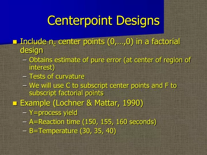
Centerpoint Designs • Include nc center points (0,…,0) in a factorial design • Obtains estimate of pure error (at center of region of interest) • Tests of curvature • We will use C to subscript center points and F to subscript factorial points • Example (Lochner & Mattar, 1990) • Y=process yield • A=Reaction time (150, 155, 160 seconds) • B=Temperature (30, 35, 40)
Centerpoint Designs 41.5 40 +1 40.340.540.740.240.6 B 0 -1 39.3 40.9 -1 0 +1 A
Centerpoint Designs • Statistics used for test of curvature
Centerpoint Designs • When do we have curvature? • For a main effects or interaction model, • Otherwise, for many types of curvature,
Centerpoint Designs • A test statistic for curvature
Centerpoint Designs • T has a t distribution with nC-1 df (t.975,4=2.776) • T>0 indicates a hilltop or ridge • T<0 indicates a valley
Centerpoint Designs • We can use sC to construct t tests (with nC-1 df ) for the factor effects as well • E.g., To test H0: effect A = 0the test statistic would be:
Follow-up Designs • If curvature is significant, and indicates that the design is centered (or near) an optimum response, we can augment the design to learn more about the shape of the response surface • Response Surface Design and Methods
Follow-up Designs • If curvature is not significant, or indicates that the design is not near an optimum response, we can search for the optimum response • Steepest Ascent (if maximizing the response is the goal) is a straightforward approach to optimizing the response
Steepest Ascent • The steepest ascent direction is derived from the additive model for an experiment expressed in either coded or uncoded units. • Helicopter II Example (Minitab Project) • Rotor Length (7 cm, 12 cm) • Rotor Width (3 cm, 5 cm) • 5 centerpoints (9.5 cm, 4 cm)
Steepest Ascent • Helicopter II Example:
Steepest Ascent • The coefficients from either the coded or uncoded additive model define the steepest ascent vector (b1 b2)’. • Helicopter II Example 2.775+.425RL-.175RW= 2.775+.425(RL*-9.5)/2.5-.175(RW*-3)= (2.775-1.615+.525) + .17RL* -.175RW*= 1.685+.17RL*-.175RW*
Steepest Ascent • With a steepest ascent direction in hand, we select design points, starting from the centerpoint along this path and continue until the response stops improving. • If the first step results in poorer performance, then it may be necessary to backtrack • For the helicopter example, let’s use (1, -1)’ as an ascent vector.
Steepest Ascent • Helicopter II Example:
Steepest Ascent • The point along the steepest ascent direction with highest mean response will serve as the centerpoint of the new design • Choose new factor levels (guidelines here are vague) • Confirm that • Add axial points to the design to fully characterize the shape of the response surface and predict the maximum.
Steepest Ascent • The axial points are chosen so that the response at each combination of factor levels is estimated with approximately the same precision. • With 9 distinct design points, we can comfortably estimate a full quadratic response surface • We usually translate and rotate X1 and X2 to characterize the response surface (canonical analysis)