Download

1 / 12
120 likes | 183 Views
Explore polynomial fitting in physics through MATLAB examples. Learn how to fit second-degree polynomials and analyze chi-square for different orders. Understand linearizing non-linear fits.

E N D
Physics 114: Lecture 17 Least Squares Fit to Polynomial Dale E. Gary NJIT Physics Department
Reminder, Linear Least Squares • We start with a smooth line of the form which is the “curve” we want to fit to the data. The chi-square for this situation is • To minimize any function, you know that you should take the derivative and set it to zero. But take the derivative with respect to what? Obviously, we want to find constants a and b that minimize , so we will form two equations:
Polynomial Least Squares • Let’s now allow a curved line of polynomial form which is the curve we want to fit to the data. • For simplicity, let’s consider a second-degree polynomial (quadratic). The chi-square for this situation is • Following exactly the same approach as before, we end up with three equations in three unknowns (the parameters a, b and c):
Second-Degree Polynomial • The solution, then, can be found from the same determinant technique we used before, except now we have 3 x 3 determinants: • You can see that extending to arbitrarily high powers is straightforward, if tedious. • We have already seen the MatLAB command that allows polynomial fitting. It is just p = polyfit(x,y,n), where n is the degree of the fit. We have used n = 1 so far.
MatLAB Example: 2nd-Degree Polynomial Fit • First, create a set of points that follow a second degree polynomial, with some random errors, and plot them: • x = -3:0.1:3; • y = randn(1,61)*2 - 2 + 3*x + 1.5*x.^2; • plot(x,y,'.') • Now use polyfit to fit a second-degree polynomial: • p = polyfit(x,y,2) prints p = 1.5174 3.0145 -2.5130 • Now overplot the fit • hold on • plot(x,polyval(p,x),'r') • And the original function • plot(x,-2 + 3*x + 1.5*x.^2,'g') • Notice that the points scatter about the fit. Look at the residuals.
MatLAB Example (cont’d): 2nd-Degree Polynomial Fit • The residuals are the differences between the points and the fit: • resid = y – polyval(p,x) • figure • plot(x,resid,'.') • The residuals appear flat and random, which is good. Check the standard deviation of the residuals: • std(resid) prints ans = 1.9475 • This is close to the value of 2 we used when creating the points.
MatLAB Example (cont’d): Chi-Square for Fit • We could take our set of points, generated from a 2nd order polynomial, and fit a 3rd order polynomial: • p2 = polyfit(x,y,3) • hold off • plot(x,polyval(x,p2),'.') • The fit looks the same, but there is a subtle difference due to the use of an additional parameter. Let’s look at the standard deviation of the new • resid2 = y – polyval(x,p2) • std(resid2) prints ans = 1.9312 • Is this a better fit? The residuals are slightly smaller BUT check chi-square. • chisq1 = sum((resid/std(resid)).^2) % prints 60.00 • chisq2 = sum((resid2/std(resid2)).^2) % prints 60.00 • They look identical, but now consider the reduced chi-square. sum((resid/std(resid)).^2)/58. % prints 1.0345 sum((resid2/std(resid2)).^2)/57. % prints 1.0526 => 2nd-order fit is preferred
Linear Fits, Polynomial Fits, Nonlinear Fits • When we talk about a fit being linear or nonlinear, we mean linear in the coefficients (parameters), not in the independent variable. Thus, a polynomial fit is linear in coefficients a, b, c, etc., even though those coefficients multiply non-linear terms in independent variable x, (i.e. cx2). • Thus, polynomial fitting is still linear least-squares fitting, even though we are fitting a non-linear function of independent variable x. The reason this is considered linear fitting is because for n parameters we can obtain n linear equations in n unknowns, which can be solved exactly (for example, by the method of determinants using Cramer’s Rule as we have done). • In general, this cannot be done for functions that are nonlinear in the parameters (i.e., fitting a Gaussian function f(x) = a exp{-[(x-b)/c]2}, or sine function f(x) = a sin[bx +c]). We will discuss nonlinear fitting next time, when we discuss Chapter 8. • However, there is an important class of functions that are nonlinear in parameters, but can be linearized (cast in a form that becomes linear in coefficients). We will now take a look at that.
Linearizing Non-Linear Fits • Consider the equation wherea and b are the unknown parameters. Rather than consider a and b, we can take the natural logarithm of both sides and consider instead the function • This is linear in the parameters ln a and b, where chi-square is • Notice, though, that we must use uncertainties si′, instead of the usual si to account for the transformation of the dependent variable:
MatLAB Example: Linearizing An Exponential • First, create a set of points that follow the exponential, with some random errors, and plot them: • x = 1:10; • y = 0.5*exp(-0.75*x); • sig = 0.03*sqrt(y); % errors proportional to sqrt(y) • dev = sig.*randn(1,10); • errorbar(x,y+dev,sig) • Now convert using log(yi) – MatLAB for ln(yi) • logy = log(y+dev); • plot(x,logy,’.’) • As predicted, the points now make a pretty good straight line. What about the errors. You might think this will work: • errorbar(x, logy, log(sig)) • Try it! What is wrong?
MatLAB Example (cont’d): Linearizing An Exponential • The correct errors are as noted earlier: • logsig = sig./y; • errorbar(x, logy, logsig) • This now gives the correct plot. Let’s go ahead and try a linear fit. Remember, to do a weighted linear fit we use glmfit(). • p = glmfit(x,logy,’normal’,’weights’,logsig); • p = circshift(p,1); % swap order of parameters • hold on • plot(x,polyval(p,x),’r’) • To plot the line over the original data: • hold off • errorbar(x,y+dev,sig) • hold on • plot(x,exp(polyval(p,x)),’r’) • Note parameters a′ = ln a = -0.6931, b′ = b = -0.75
Summary • Use polyfit() for polynomial fitting, with third parameter giving the degree of the polynomial. Remember that higher-degree polynomials use up more degrees of freedom (an nth degree polynomial takes away n + 1 DOF). • A polynomial fit is still considered linear least-squares fitting, despite its dependence on powers of the independent variable, because it is linear in the coefficients (parameters). • For some problems, such as exponentials, , one can linearize the problem. Another type that can be linearized is a power-law expression, as you will do in the homework. • When linearizing, the errors must be handled properly, using the usual error propagation equation, e.g.