Download
1 / 51
510 likes | 524 Views
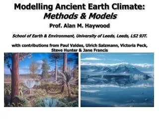
Modelling Ancient Earth Climate. Alan Haywood School of Earth & Environment, University of Leeds With thanks to Paul Valdes, Jane Francis, Dan Lunt, Vicky Peck, Mark Williams and Harry Dowsett. CONTENT: Rationale Models and Modelling Eocene/Oligocene - Bipolar Glaciation?

E N D
Modelling Ancient Earth Climate Alan Haywood School of Earth & Environment, University of Leeds With thanks to Paul Valdes, Jane Francis, Dan Lunt, Vicky Peck, Mark Williams and Harry Dowsett
CONTENT: • Rationale • Models and Modelling • Eocene/Oligocene - Bipolar Glaciation? • Estimates of Earth System Sensitivity - Climate Vs Earth System Sensitivity - The Pliocene - Palaeo estimates of Earth System Sensitivity
Motto and Philosophy Everything comes to those who wait Occam's razor: if all things are equal then the simplest solution is probably correct
Why? • Understand climate dynamics • Test Earth System Models
Primary Research Focus in Climate Change Science • Simulation of the historical or near-historical record • Analysis of the observed record of variability • Projection for the next 100 years Greatest Strengths Spatial and temporal character of the observations. Measurement of physical quantities that define the state of the atmosphere and ocean. Greatest Weaknesses Sense of change. Sense of the integration of the Earth System.
In contrast: A Research Focus in Earth History Greatest Strengths Spectacular sense of change (Furry Alligator Syndrome) True integrated system response Greatest Weaknesses Proxies rather than state variables Limited spatial and temporal resolution “The greatest weaknesses in a research focus on the modern record are the greatest strengths of Earth System History”
Climate History
General Circulation Models Model needs to simulate albedo, emissivity and general circulation. Use “first principles” Newton's Laws of Motion 1st Law of Thermodynamics Conservation of Mass and Moisture Hydrostatic Balance Ideal Gas Law
Aerosols: Dust and Sulphates Regional Model: High Resolution Cryosphere-Lithosphere Model Atmospheric General Circulation Model Atmospheric Chemistry Land Surface Hydrology Ocean Carbon Cycle Ocean General Circulation Model Terrestrial Carbon Cycle Components of an Earth System Model
Development of Met. Office Climate Models ATMOSPHERE OCEAN ICE SULPHUR CARBON CHEMISTRY LAND Present ATMOSPHERE OCEAN ICE SULPHUR 1999 CARBON LAND 1997 ATMOSPHERE OCEAN ICE SULPHUR LAND 1992 ATMOSPHERE OCEAN ICE LAND Component models are constructed off-line and coupled in to the climate model when sufficiently developed ATMOSPHERE OCEAN LAND 1990 ATMOSPHERE 1985 LAND ATMOSPHERE 1960s
HadCM3 GCM Atmospheric resolution: 3.75 by 2.5 degrees 19 Atmospheric Levels Ocean resolution :1.25 by 1.25 20 Ocean Levels
30km 19 levels in atmosphere 2.5 lat 3.75 long THE HADLEYCENTRETHIRDCOUPLEDMODEL -HadCM3 no flux adjustments 1.25 1.25 20 levelsin ocean -5km
Greenhouse to Icehouse transition First permanent ice sheet on Antarctica pCO2 decrease Sea level fall of 55-80 m CCD deepened by ~1 km/carbon cycle reorganisation Initiation of NADW Opening of tectonic gateways Biotic overturn in plants and animals >8 °C cooling in North America/ aridification of the Himalayas How much ice? Zachos et al., 2001
Ferns Dickinsonia antarctica Fossil Cladophlebis
3D preserved conifer branches in concretions Araucaria araucana
Nothofagaceae How much ice? Fossil Nothofagaceae Nothofagus cunninghamii
Site 1263 1 0.5 ‰ 100 kyr 2 0.7 ‰ 30 kyr ODP Site 1263 ~1.2 ‰ Riesselman et al. 2007 O. umbonatus image from Douglas, 1973
But what does it represent? Modern Antarctic ice vol.* Model simulation Observed sea level fall* At least 3 °C? More ice? Or both? How much Dice volume? How much Dtemperature? *10 m sea level fall = 0.1 ‰ 1 °C = 0.22 ‰
Benthic d18O = Ice growth + cooling ? INDIAN PACIFIC ATLANTIC Late Eocene INDIAN PACIFIC ATLANTIC Early Oligocene In the Earliest Oligocene…. NADW formation was just beginning Antarctica was the principal source of deep water formation Cooling expected to be transmitted to deep-waters
Benthic Mg/Ca suggests no cooling? ODP Site 1218 Pacific ODP Site 1218 @ ~3800 m paleodepth (similar to CCD) ~2 °C warming Lear et al., 2004 South Atlantic DSDP Site 522 @ ~3000 m paleodepth (1 km above CCD) no change in temperature Lear et al., 2000 DSDP Site 522
Will we find cooling at shallower sites (?) South Atlantic ODP Site 1263 Paleodepth ~ 2.1 km Paleo-lysocline ~ 3.8 km Paleo-CCD ~ 4.2 km prior to CCD deepening at E-O O • Assumptions/hopes • Similar CO32- gradient • 2. Mg/Ca response less at high CO32- concentrations Modern Atlantic estimates after Anderson and Archer, 2002
Modelling approach Aim Predict effect of an Antarctic ice sheet on global ocean in Early Oligocene Model parameters HadCM3L 2 x pre-industrual pCO2 Solar constant –0.3 % Paleogeography of Rupelian (Markwick et al., 2001) Vegetation cover predicted by TRIFFID
Effect of growing an East Antarctic ice sheet… Model initially run for 800 years Ocean temperature at 3962 m (°C) E. Oli - E. Oli Ocean temperature at 5 m (°C) E. Oli - E. Oli Ann xboya-xboyc Ann xboya-xboyc -3.0 -2.0 -1.0 -0.8 -0.6 -0.4 -0.2 0.2 0.4 0.6 0.8 1.0 2.0 3.0 -3.0 -2.0 -1.0 -0.8 -0.6 -0.4 -0.2 0.2 0.4 0.6 0.8 1.0 2.0 3.0
But, model did not reach equilibrium… Upper ocean integral of temperature (<300 m) Model with modern Antarctic ice volume ~ 0.7 °C cooling
But, model did not reach equilibrium… Lower ocean integral of temperature (>300 m) Model with modern Antarctic ice volume ~ 0.75 °C cooling
Model run extended to 2200 years Ocean temperature at 5 m (°C) E. Oli - E. Oli Ocean temperature at 3962 m (°C) E. Oli - E. Oli Ann xboya1-xboyc1 Ann xboya1-xboyc1 -3.0 -2.0 -1.0 -0.8 -0.6 -0.4 -0.2 0.2 0.4 0.6 0.8 1.0 2.0 3.0 -3.0 -2.0 -1.0 -0.8 -0.6 -0.4 -0.2 0.2 0.4 0.6 0.8 1.0 2.0 3.0
Surface ocean response to ice sheet Ocean temperature at 5 m (°C) E. Oli - E. Oli Ann xboya-xboyc 2200 yr After 800 years -3.0 -2.0 -1.0 -0.8 -0.6 -0.4 -0.2 0.2 0.4 0.6 0.8 1.0 2.0 3.0 O ODP Site 1263 Ocean temperature at 5 m (°C) E. Oli - E. Oli Ann xboya1-xboyc1 After 2200 years -3.0 -2.0 -1.0 -0.8 -0.6 -0.4 -0.2 0.2 0.4 0.6 0.8 1.0 2.0 3.0
Upper ocean approaching equilibrium Upper ocean integral of temperature (<300 m) Model with modern Antarctic ice volume ~ 1 °C cooling
Deep ocean response to ice sheet Ocean temperature at 3962 m (°C) E. Oli - E. Oli Ann xboya-xboyc After 800 years -3.0 -2.0 -1.0 -0.8 -0.6 -0.4 -0.2 0.2 0.4 0.6 0.8 1.0 2.0 3.0 O ODP Site 1263 Ocean temperature at 3962 m (°C) E. Oli - E. Oli Ann xboya1-xboyc1 After 2200 years -3.0 -2.0 -1.0 -0.8 -0.6 -0.4 -0.2 0.2 0.4 0.6 0.8 1.0 2.0 3.0
Lower ocean approaching equilibrium? Lower ocean integral of temperature (>300 m) Model with modern Antarctic ice volume >1.3 °C cooling
Benthic d18O = Ice growth + cooling Observed sea level fall* Modern Antarctic ice vol.* Model ? How much Dice volume? How much Dtemperature? *10 m sea level fall = 0.1 ‰ 1 °C = 0.22 ‰
How much did deep waters cool? Upper ocean integral of temperature (<300 m) ?
Findings to date… Model predicts cooling of deep ocean in response to Antarctic glaciation in the Early Oligocene Response in surface ocean temperature is spatially heterogeneous, but at the site of 1263 the model is consistent with SST records from 1263 Deep ocean is predicted to have cooled by 0.8 °C within 2200 years of Antarctic glaciation Cooling may be significantly more by the time the model has reached equilibrium…extreme ice volumes were not a feature of the Eocene-Oligocene transition
Climate Versus Earth System Sensitivity Constraining Earth System sensitivity “Equilibrium climate sensitivity refers to the equilibrium change in global mean surface temperature following a doubling of the atmospheric (equivalent) CO2 concentration (Charney sensitivity)”. Estimates based around components of the Earth system that respond quickly (atmosphere, surface ocean) and neglects feedbacks linked to changing deep ocean circulation, vegetation distribution and ice sheets, which can be referred to as Earth System Sensitivity. IPCC 2007: 2 to 4.5°C. Best estimate is 3°C. Is this supported by palaeoclimatology? How different is ESS?
Dowsett et al. (1999) The mid-Pliocene and causes of mid-Pliocene warmth Published Mechanisms: Trace gases (Raymo et al., 1996) Ocean heat transport (Dowsett et al., 1992) Palaeogeography (Rind & Chandler, 1991) Lisiecki & Raymo (2005) ENSO dynamics (Philander & Federov, 2003)
Palaeobotanical data The mid-Pliocene: a different world Vegetation… Salzmann et al. (2008) Ice… Orography… Fission track, Parrish et al, 2007 Dowsett and Cronin (1990)
Mid-Pliocene Control and Data/Model Comparisons HadCM3 Total = 3.3oC Haywood and Valdes (2004) Salzmann et al. (2009)
An Ensemble Modelling Approach (changes from the pre-industrial to mid-Pliocene) Causes of Pliocene warmth….
An Ensemble Modelling Approach (changes from the pre-industrial to mid-Pliocene) Be cautious of the order of change…
= 0.7˚C = 0.7˚C = 1.6˚C = 0.4˚C Relative Contribution to mid-Pliocene Warmth Total Warming = 3.3°C
Calculation of Earth System Sensitivity • Mid-Pliocene warmth (3.3oC) was due to … • Higher CO2 – 1.5oC (47%) • (2) Modified vegetation – 0.8oC (26%) • (3) Less ice – 0.1oC (4%) • (4) Lower orography – 0.8oC (24%) • Implications for the future… • (ignoring the orographic variations) • Just CO2, temp change of 1.5oC - Climate Sensitivity~3oC • CO2, veg and ice, temp change of 2.5oC - Earth System Sensitivity ~5oC
Sensitivity to Boundary Condition Implementation within the GCM Total = 3.3oC CO2 = 1.5oC veg= 0.8oC orog = 0.8oC ice= 0.1oC CO2 = 1.4oC veg= 1.1oC orog = 0.6oC ice= 0.1oC