Heteroscedasticity

1. Heteroscedasticity

2. Heteroscedasticity • Our 40-household example • Total household food expenditure • FD_EXP=β0+β1INC

3. Heteroscedasticity • Our 40-household example • As INC , the errors have a tendency to increase → maybe var(et)  with INC

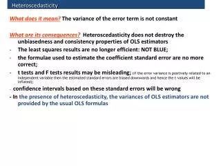
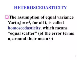
4. Heteroscedasticity • What are the economic implications of this non-constant error variance? • → for low income levels, food expenditures clustered close to the mean function, E(yt). • Food expenditures almost totally explained by income • → for high income levels, food expenditures can deviate more from the mean function • Many other factors determine food expenditures • Is σt2 = h(INCt)?

5. Heteroscedasticity • Yt=Xtβ+etE[e′e]=2Ψ • Ψis diagonal matrix • Diagonal elements are not identical across observations • σ2i not all equal (some could be)

6. Heteroscedasticity • The most general heteroscedastic specification: • Φ=diag(σ21, σ22,… σ2T) • Can not estimate T+K parameters with only T observations. We need to reduce the number of parameters. T additional parameters to est.

7. Heteroscedasticity • Heteroscedasticity Example #1 • Assume we partition data into subsets of observations. Each subset has a different variance but within the subset of observations error variances are the same • T=Ta+Tb • Yi,ei→(Tix1) Xi→(Ti x K) X e Y Assume σ2=1→ Ψ = Φ

8. Heteroscedasticity • Heteroscedasticity Example #1

9. Heteroscedasticity • Heteroscedasticity Example #1

10. Heteroscedasticity • Remember βG=(X'Φ-1X)-1 X'Φ-1Y =(X'(σ2Ψ)-1X)-1X'(σ2Ψ)-1Y =(σ-2X'Ψ-1X)-1σ-2X'Ψ-1Y =σ2σ-2 (X'Ψ-1X)-1X'Ψ-1Y =(X'Ψ-1X)-1 X'Ψ-1Y • Under current structure→ X' (K x T) (T x 1) (T x T)

11. Heteroscedasticity • FGLS Estimation Procedure • Obtain LS parameter estimates for each sub-sample βsi=(Xi'Xi)-1Xi'Yi (i=a, b) →esi=Yi-Xiβsi (a consistent estimator of ei) • Estimate 2u,i • Construct estimate of Ψ matrix • Obtain FGLS estimate of  (T x T)

12. Heteroscedasticity • FGLS Estimation Procedure Ψ-1 ΣβFG=σ2(X'Ψ-1X)-1 Assume σ2=1

13. Heteroscedasticity • Are 2a and 2b actually different? • Variation of the Goldfeld-Quandt Test • JHGLL, CH. 9:362-363 Greene, Ch 11. pp 223 • H0: 2a= 2b = σ2 H1: 2a≠2b • Remember if we have two RV’s distributed χ2(r1) and χ2(r2) true unknown value

14. Heteroscedasticity true unknown values • If H0 true: σ2i (i=a,b) are independent due to being estimated from separate datasets which are independent of one another Ratio of 2 indep. χ2 cancel out under H0 • H0: 2a= 2b = σ2 H1: 2a≠ 2b

15. Heteroscedasticity H0: 2a= 2b = σ2 H1: 2a≠ 2b • Goldfeld-Quandt Test Procedure • Choose =Pr(Type I Error) = Pr(Rejecting H0|H0 True) • Given H1 find cL and cU where: • Reject H0 if • Do Not Reject H0 if • Two-sided F-Test (use Gauss Code to determine FCL, FCU given that no book values available)

16. Heteroscedasticity • 40-Household food expenditure example • As Income ↑, deviation from regression line tends to ↑ • Not consistent w/ constant variance assumption

17. Heteroscedasticity • 40-Household food expenditure example • Goldfeld-Quandt Test • Sort data by income level • Highest first • 20 obs. in each sample • Obtain separate estimates of σu2 • H0: σ2High Inc= σ2Low Inc • Undertake F-tests • 1-Tail Test H1: σ2High Inc> σ2Low Inc • 2-Tail Test H1: σ2High Inc ≠σ2Low Inc

18. Heteroscedasticity • Australian Wheat Supply Example • Qs=f(price, technology, weather) • 26 yrs. of aggregate time-series data on wheat quantity marketed and price received • After year 13, new wheat varieties introduced that are drought tolerant→lower variance in wheat yields (mean neutral)

19. Heteroscedasticity • Australian Wheat Supply Example • Qs=f(price, technology, weather) • Variance of residuals tend to decrease after year 13

20. Heteroscedasticity Flow Chart for GLS Code (GLS_SEP_2.GAS) Data: All Obs Data Sample 1 Data Sample 2 CRM CRM σu12 σu22 GQ Test ΨFG GLS

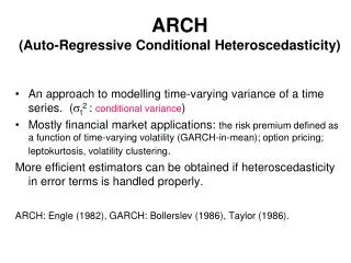
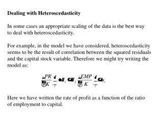
21. Heteroscedasticity • Australian Wheat Supply Example • Qs=f(price, technology) • Overview of GAUSS Code • Results of GQ test • GLS Results • Heteroscedasticity Example #2 • In the food example we saw evidence that the error variance is positively related to income • E(etet') =cov(etes)=0 for t≠s =var(et)=σ2t=h(inct) for t=s

22. Heteroscedasticity • Heteroscedasticity Example #2 • In general, lets define the index: It=0+ 1z1t+…+ DzDt where t2 = h(It) • Need to estimate only D+1 additional parameters (Note my notation is different the JHGLL who have S additional paramaters including intercept term) • Would like the above function h(It) to always generate a positive value given that t2 > 0 exog. variable

23. Heteroscedasticity It=0+ 1z1t+…+ DzDt • Heteroscedasticity Example #2 • t2 = exp(It) = exp(Ztg) > 0 • Referred to as Multiplicative Heteroscedasticity • t2 =exp(Ztγ)=exp(0)exp(Zt**) = 2exp(Zt* *) • 2 = exp(0) • *=[γ1, γ2, …,γD] • Z* does not contain a constant vector while Z does • Need to estimate D+1 parameters instead of T σt2’s • Still generate T σt2’s • Lets develop a FGLS estimator of σt2 using above structure • Two-step approach • Later on use ML techniques

24. Heteroscedasticity • FGLS estimator using above structure • Use CRM to obtain consistent estimates of error term. That is, βs=(X'X)-1X′y continues to be a consistent estimator of β even with multiplicative heteroscedasticity • es=y – Xβs is consistent • ln(σt2)= Zt given t2=exp(Ztγ) • ln(est2)+ln(σt2)= ln(est2)+ Ztγ • ln(est2) = Ztγ+vt • vt ≡ ln(est2)-ln(σt2) • est obtained from CRM • γs=(Z'Z)-1Z' ln(est2) CRM estimate dependent variable

25. Heteroscedasticity ln(e2s) • γs=(Z'Z)-1Z'(Zγ+v) =(Z'Z)-1Z'Zγ+ (Z'Z)-1Z'v = γ + (Z'Z)-1Z'v • The properties of γs depend on the properties of v, the “combined” error term • Unfortunately, vt does not have nice properties (i.e., non-zero mean, heteroscedastic and autocorrelated) • Some asymptotic results • γ0s, the estimated intercept • inconsistent • inconsistency of -1.2704 • Remaining elements of γ are consistent

26. Heteroscedasticity • Consistent parameter vector obtained via the following: • 4.9348(Z'Z)-1 approximates the cov. matrix of γ asymptotically • FGLS estimator of β: True Value

27. Heteroscedasticity • FGLS estimator using above structure coef. obtained from pseudo-regression

28. Heteroscedasticity • FGLS estimator using above structure where Zt*=(zt1, zt2,…,ztD) no intercept coef. obtained from pseudo-regression

29. Heteroscedasticity • FGLS estimator using above structure • Given our multiplicative specification: • Note the negative sign on Z*t • βFG depends only on the consistently estimated elements of γ

30. Heteroscedasticity • Testing for heteroscedasticity • Multiplicative Hetero.: 2 test • Goldfeld-Quandt test • Breusch-Pagan test • White’s test

31. Heteroscedasticity Flowchart of the Multiplicative Heterscedasticity 2-step Model CRM of Full Model Y X es Factors Impacting Variance, Z Pseudo- regression γs Build Ψe Correct Σβs GLS Estimate of β’s GLS Est. of Σβs

32. Heteroscedasticity • Lets review some GAUSS code that estimates the 2-step (Aitken) estimator for the multiplicative heteroscedasticity model • Table 9.1, JHGLL, p.374 • yt=β1 + β2Xt2 + β3Xt3 + et • E(et)=0, E(et2)=σt2 σt2 = exp{α1+ α2Xt2} • The above code reports the initial CRM results along with GLS results

33. Heteroscedasticity • In terms of coefficient covariance matrices: • Note that the above code prints out the correct CRM covariance matrix: Σβ=σ2(X′X)-1X′ΨX(X′X)-1 • The GLS covariance matrix is used: ΣβG= σ2(X′Ψ-1X)-1 • Compare the diagonal elements of these two matrices to verify that GLS is relatively more efficient than CRM