Download
1 / 89
890 likes | 904 Views
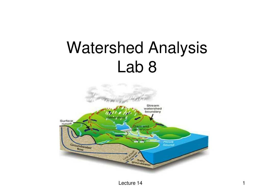
Learn how to create raster drainage basins and process DEM data for watershed analysis. Understand resampling and flow direction methods for accurate hydrological modeling.

E N D
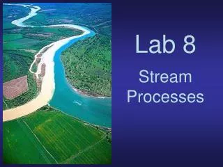
Watershed AnalysisLab 8 Lecture 14
Basin • Creates a raster delineating all drainage basins. • All cells in the raster will belong to a basin, even if that basin is only one cell. • The drainage basins are delineated within the analysis window by identifying ridge lines between basins. • The input flow direction raster is analyzed to find all sets of connected cells that belong to the same drainage basin. Lecture 14
The drainage basins are created by locating the pour points at the edges of the analysis window (where water would pour out of the raster), as well as sinks, then identifying the contributing area above each pour point. This results in a raster of drainage basins. Lecture 14
Lab 8 Data • Report Sheet is on the Website with the instructions, • Three files will be downloaded: • 2 from NY Gis Clearinghouse • 1 from Cornell University • The DEM will be obtained from ArcGIS online. Lecture 14
Step 13 – DEM (30-second Arc) Lecture 14
Measuring in Arc-Seconds • Some USGS DEM data is stored in a format that utilizes three, five, or 30 arc-seconds of longitude and latitude to register cell values. • The geographic reference system treats the globe as if it were a sphere divided into 360 equal parts called degrees. Lecture 14
Each degree is subdivided into 60 minutes. Each minute is composed of 60 seconds. • Arc-seconds of latitude remain nearly constant, while arc-seconds of longitude decrease in a trigonometric cosine-based fashion as one moves toward the earth's poles. Lecture 14
Processing of DEM • Raster clip – To the buffered park boundry. • Raster projection – from Geographic to UTM Zone 18N, NAD83 • Resample – Bilinear Interpolation • Change the cell size – from 30 second arc to 30 meters, Lecture 14
Raster Geometry and Resampling • Data must often be resampled when converting between coordinate systems or changing the cell size of a raster data set. • Common methods: • Nearest neighbor • Bilinear interpolation • Cubic convolution Lecture 14
ResamplingBilinear Interpolation Distance weighted averaging Lecture 14
Step 17 - DEM Lecture 14
DEM_UTM83 FlowDir Sinks Filled FlowDir2 Watershed FlowAcc Source Stream Link Reclass Con Net Hydrological Modeling Lecture 14
Flow Direction • Creates a raster of flow direction from each cell to its steepest downslope neighbor. Lecture 14
flowDir Lecture 14
Sinks • A sink is a cell or set of spatially connected cells whose flow direction cannot be assigned one of the eight valid values in a flow direction raster. • This can occur when all neighboring cells are higher than the processing cell or when two cells flow into each other, creating a two-cell loop. • To create an accurate representation of flow direction and, therefore, accumulated flow, it is best to use a dataset that is free of sinks. • A digital elevation model (DEM) that has been processed to remove all sinks is called a depressionless DEM. From ArcGIS 10 Desktop Help Lecture 14
High pass filters Return: • Small values when smoothly changing values. • Large positive values when centered on a spike • Large negative values when centered on a pit Lecture 14
Lecture 14 35.7
Step 18 - Sinks Lecture 14
Fill • Fills sinks in a surface raster to remove small imperfections in the data. • Sinks (and peaks) are often errors due to the resolution of the data or rounding of elevations to the nearest integer value. Lecture 14
Step 19 - Fill Lecture 14
flowDir2 Lecture 14
Flow Accumulation Lecture 14 From ArcGIS 10 Desktop Help
Flow AccumulationStep 21 before inverting Lecture 14
After inverting Lecture 14
Conditional • The results of Flow Accumulation can be used to create a stream network by applying a threshold value to select cells with a high accumulated flow. • For example, the procedure to create a raster where the value 1 represents the stream network on a background of NoData could use one of the following: • Perform a conditional operation with the Con tool with the following settings: • Input conditional raster : Flowacc • Expression : Value > 50000 • Input true raster or constant : 1 Lecture 14 From ArcGIS 10 Desktop Help
Net50K Lecture 14
Stream Link • Assigns unique values to sections of a raster linear network between intersections. • Links are the sections of a stream channel connecting two successive junctions, a junction and the outlet, or a junction and the drainage divide. • Links are the sections of a stream channel connecting two successive junctions, a junction and the outlet, or a junction and the drainage divide. Lecture 14 From ArcGIS 10 Desktop Help
Watershed 50K Lecture 14
Watershed Clipped to Park Boundry Lecture 14
Lecture 14Data Quality Issues Ch. 14 Lecture 14 31
Introduction • Spatial data and analysis standards are important because of the range of organizations producing and using spatial data, and the amount of data transferred between these organizations. • There are several types of standards: • Data standards • Interoperability standards • Analysis standards • Professional and certification standards Lecture 14
Introduction (continued) • National and international standards organizations are important in defining and maintaining geospatial standards: • Federal Geographic Data Committee (FGDC) which focuses on the national spatial data infrastructure (www.fgdc.gov) • International Spatial Data Standards Commission which is a clearing house and gateway for international standards • Open Geospatial Consortium (OGC) which is developing interoperability standards. Web Mapping Service (WMS) standards are an example. Lecture 14
The Geospatial Competency Model Lecture 14
GIS Professional Certification URISA is the founding member of the GIS Certification Institute, the organization that administers professional certification for the field and is dedicated to advancing the industry. The minimum number of points needed to become a certified GIS Professional as detailed in the three point schedules given below is 150 points. Thus, all applicants are expected to document achievements valued at a minimum of 150 points. To ensure that applicants have a broad foundation, specific minimums in each of the three achievement categories must be met or exceeded. These minimums are as follows: The additional 52 points can be counted from any of the three categories. Lecture 14 36
University Certificates • UMM – undergraduate • USM undergrad/grad • UM – graduate • Penn State – graduate • University of Denver • University of Southern California • George Mason University Lecture 14
Spatial Data Standards • Data – measurements and observations • Data quality – a measure of the fitness for use of data for a particular task (Chrisman, 1994). • It is the responsibility of the user to insure that the data is fit for the task. • Metadata – data about the data Lecture 14 39
Spatial Data Standards Spatial Data Standards – methods for structuring, describing and delivering spatially-referenced data. Media Standards – the physical form of the data (CD/download etc). Format Standards – specify data file components and structures. These standards aid in data transfer. Spatial Data Accuracy Standards–document the quality of the positional and attribute accuracy. Document Standards – define how we describe spatial data. Lecture 14 40
GIS Is Not Perfect A GIS cannot perfectly represent the world for many reasons, including: • The world is too complex and detailed. • The data structures or models (raster, vector, or TIN) used by a GIS to represent the world are not discriminating or flexible enough. • We make decisions (how to categorize data, how to define zones) that are not always fully informed or justified. • It is impossible to make a perfect representation of the world, so uncertainty is inevitable • Uncertainty degrades the quality of a spatial representation Lecture 14 41
Concepts Related to Data Quality • Related to individual data sets: • Errors – flaws in data • Accuracy – the extent to which an estimated value approaches the true value. • Precision – the recorded level of detail of your data. • Bias – the systematic variation of the data from reality. Lecture 14 42
Lecture 14 43
Concepts Related to Data Quality • Related to source data: • Resolution – the smallest feature in the data set that can be displayed. • Generalization- simplification of objects in the real world to produce scale models and maps. Lecture 14 44
Resolution and generalization of raster datasets Lecture 14 45
Scale-related generalization Lecture 14 46
Data Sets Used for Analysis Must be: • Complete – spatially and temporally • Compatible – same scale, units of measure, measurement level • Consistent – both within and between data sets. • And Applicable for the analysis being performed. Lecture 14 47
A Conceptual View of Uncertainty Real World Conception Source Data, Measurements & Representation Data conversion and Analysis error propagation Lecture 14 48 Result
Uncertainty in The Conception of Geographic Phenomena Many spatial objects are not well defined or their definition is to some extent arbitrary, so that people can reasonably disagree about whether a particular object is x or not. There are at least four types of conceptual uncertainty • Spatial uncertainty • Vagueness • Ambiguity • Regionalization problems Lecture 14 49
Spatial uncertainty Spatial uncertainty occurs when objects do not have a discrete, well defined extent. • They may have indistinct boundaries. • They may have impacts that extend beyond their boundaries. • They may simply be statistical entities. • The attributes ascribed to spatial objects may also be subjective. Lecture 14 50