Download
1 / 42
840 likes | 2.16k Views
LECTURE 3 Introduction to Linear Regression and Correlation Analysis. 1 Simple Linear Regression 2 Regression Analysis 3 Regression Model Validity. Goals. After this, you should be able to: Interpret the simple linear regression equation for a set of data

E N D
LECTURE 3Introduction to Linear Regression and Correlation Analysis 1 Simple Linear Regression 2 Regression Analysis 3 Regression Model Validity
Goals After this, you should be able to: • Interpret the simple linear regression equation for a set of data • Use descriptive statistics to describe the relationship between X and Y • Determine whether a regression model is significant
Goals (continued) After this, you should be able to: • Interpret confidence intervals for the regression coefficients • Interpret confidence intervals for a predicted value of Y • Check whether regression assumptions are satisfied • Check to see if the data contains unusual values
Introduction to Regression Analysis • Regression analysis is used to: • Predict the value of a dependent variable based on the value of at least one independent variable • Explain the impact of changes in an independent variable on the dependent variable Dependent variable: the variable we wish to explain Independent variable: the variable used to explain the dependent variable
Simple Linear Regression Model • Only one independent variable, x • Relationship between x and y is described by a linear function • Changes in y are assumed to be caused by changes in x
Types of Regression Models Positive Linear Relationship Relationship NOT Linear Negative Linear Relationship No Relationship
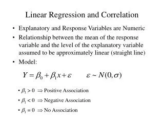
Population Linear Regression The population regression model: Random Error term, or residual Population SlopeCoefficient Population y intercept Independent Variable Dependent Variable Linear component Random Error component
Linear Regression Assumptions • The underlying relationship between the x variable and the y variable is linear • The distribution of the errors has constant variability • Error values are normally distributed • Error values are independent (over time)
Population Linear Regression y Observed Value of y for xi εi Slope = β1 Predicted Value of y for xi Random Error for this x value Intercept = β0 x xi
Estimated Regression Model The sample regression line provides an estimate of the population regression line Estimated (or predicted) y value Estimate of the regression intercept Estimate of the regression slope Independent variable
Interpretation of the Slope and the Intercept • b0 is the estimated average value of y when the value of x is zero • b1 is the estimated change in the average value of y as a result of a one-unit change in x
Finding the Least Squares Equation • The coefficients b0 and b1 will be found using computer software, such as Excel’s data analysis add-in or MegaStat • Other regression measures will also be computed as part of computer-based regression analysis
Simple Linear Regression Example • A real estate agent wishes to examine the relationship between the selling price of a home and its size (measured in square feet) • A random sample of 10 houses is selected • Dependent variable (y) = house price in $1000 • Independent variable (x) = square feet
Regression output from Excel – Data – Data Analysis or MegaStat – Correlation/ regression • MegaStat – Correlation/ regression
MegaStatOutput The regression equation is:
Graphical Presentation • House price model: scatter plot and regression line Slope = 0.10977 Intercept = 98.248
Interpretation of the Intercept, b0 • b0 is the estimated average value of Y when the value of X is zero (if x = 0 is in the range of observed x values) • Here, houses with 0 square feet do not occur, so b0 = 98.24833 just indicates the height of the line.
Interpretation of the Slope Coefficient, b1 b1 measures the estimated change in Yas a result of a one-unit increase in X • Here, b1 = .10977 tells us that the average value of a house increases by .10977($1000) = $109.77, on average, for each additional one square foot of size
Least Squares Regression Properties • The simple regression line always passes through the mean of the y variable and the mean of the x variable • The least squares coefficients are unbiased estimates of β0 and β1
Coefficient of Determination, R2 The percentage of variability in Y that can be explained by variability in X. Note: In the single independent variable case, the coefficient of determination is where: R2 = Coefficient of determination r = Simple correlation coefficient
Examples ofR2 Values y R2 = 1, correlation = -1 Perfect linear relationship between x and y: 100% of the variation in y is explained by variation in x x R2 = 1 y x R2 = 1, correlation = +1
Examples of Approximate R2 Values y 0 < R2 < 1, correlation is negative Weaker linear relationship between x and y: Some but not all of the variation in y is explained by variation in x x y 0 < R2 < 1, correlation is positive x
Examples of Approximate R2 Values R2 = 0 y No linear relationship between x and y: The value of Y does not depend on x. (None of the variation in y is explained by variation in x) x R2 = 0
Excel Output 58.08% of the variation in house prices is explained by variation in square feet The correlation of .762 shows a fairly strong direct relationship. The typical error in predicting Price is 41.33($000) = $41,330
Inference about the Slope: t Test • t test for a population slope • Is there a linear relationship between x and y? • Null and alternative hypotheses • H0: β1 = 0 (no linear relationship) • Ha: β1 0 (linear relationship does exist) • Obtain p-value from ANOVA or across from the slope coefficient (they are the same in simple regression)
Inference about the Slope: t Test (continued) Estimated Regression Equation: The slope of this model is 0.1098 Does square footage of the house affect its sales price?
H0: β1 = 0 Ha: β1 0 Inferences about the Slope: tTest Example P-value From Excel output: Decision: Conclusion: Reject H0 We can be 98.96% confident that square feet is related to house price.
Regression Analysis for Description Confidence Interval Estimate of the Slope: Excel Printout for House Prices: We can be 95% confident that house prices increase by between $33.74 and $185.80 for a 1 square foot increase.
Estimates of Expected yfor Different Values of x The relationship describes how x impacts your estimate from y y yp y y = b0 + b1x x xp x
Interval Estimates for Different Values of x Prediction Interval for an individual y, given xpThe father from x the less accurate the prediction. y y y = b0 + b1x x xp x
Example: House Prices Estimated Regression Equation: Predict the price for a house with 2000 square feet
Example: House Prices (continued) Predict the price for a house with 2000 square feet: The predicted price for a house with 2000 square feet is 317.85($1,000s) = $317,850
Estimation of Individual Values: Example Prediction Interval Estimate for y|xp Find the 95% confidence interval for an individual house with 2,000 square feet Predicted Price Yi = 317.85 ($1,000s) = $317, 850 MegaStat will give both the predicted value as well as the lower and upper limits The prediction interval endpoints are from $215,503 to $420,065. We can be 95% confident that the price of a 2000 ft2 home will fall within those limits.
ResidualAnalysis • Purposes • Check for linearity assumption • Check for the constant variability assumption for all levels of predicted Y • Check normal residuals assumption • Check for independence over time • Graphical Analysis of Residuals • Can plot residuals vs. x and predicted Y • Can create NPP of residuals to check for normality (or use Skewness/Kurtosis) • Can check D-W statistic to confirm independence
Residual Analysis for Linearity y y x x x x residuals residuals Not Linear Linear
Residual Analysis for Constant Variance y y x x Ŷ Ŷ residuals residuals Constant variance Non-constant variance
ResidualAnalysis for Normality • Can create NPP of residuals to check for normality. If you see an approximate straight line residuals are acceptably normal. You can also use Skewness/Kurtosis. If both are within + 1 the residuals are acceptably normal ResidualAnalysis for Independence • Can check D-W statistic to confirm independence. If D-W statistic is greater than 1.3 the residuals are acceptably independent. Needed only if the data is collected over time.
Checking Unusual Data Points • Check for outliers from the predicted values (studentized and studentized deleted residuals do this; MegaStat highlights in blue) • Check for outliers on the X-axis; they are indicated by large leverage values; more than twice as large as the average leverage. MegaStat highlights in blue. • Check Cook’s Distance which measures the harmful influence of a data point on the equation by looking at residuals and leverage together. Cook’s D > 1 suggests potentially harmful data points and those points should be checked for data entry error. MegaStat highlights in blue based on F distribution values.
Patterns of Outliers • a). Outlier is extreme in both X and Y but not in pattern. The point is unlikely to alter regression line. • b). Outlier is extreme in both X and Y as well as in the overall pattern. This point will strongly influence regression line • c). Outlier is extreme for X nearly average for Y. The further it is away from the pattern the more it will change the regression. • d). Outlier extreme in Y not in X. The further it is away from the pattern the more it will change the regression. • e). Outlier extreme in pattern, but not inX or Y.Slope may not be changed much but intercept will be higher with this point included.
Summary • Introduced simple linear regression analysis • Calculated the coefficients for the simple linear regression equation • measures of strength (r, R2and se)
Summary • Described inference about the slope • Addressed prediction of individual values • Discussed residual analysis to address assumptions of regression and correlation • Discussed checks for unusual data points (continued)