Download
1 / 36
360 likes | 431 Views
First Measurement of Helicity Distributions from Proton-Proton Collisions at the CERN Large Hadron Collider using the CMS Detector. Irakli Chakaberia Final Examination April 28, 2014.

E N D
First Measurement of Helicity Distributions from Proton-Proton Collisions at the CERN Large Hadron Collider using the CMS Detector IrakliChakaberia Final Examination April 28, 2014
Our Picture of Particle Physics: A Quantum Field Theory of Quarks and Leptons Interacting via Gauge Bosons
Helicity • Helicity: the projection of spin onto the direction of motion of the particle • The helicity operator is rotationally invariant thus very convenient for the calculations of angular distributions • Angular distributions allow for a more complete description of scattering processes
Developing new electronics parts for the upgrade Commissioning the pixel detector
WebBased Monitoring of the CMS Detector • The analysis described above requires good data; which, on its side, requires good detector and good monitoring/certification. • I had an opportunity to develop such tools. FillReport DataSummary CMS PageZero CMS Page1
Zγproduction is sensitive to new physical interactions forbidden in the standard model. • A helicity analysis provides sensitivity to interference terms between different helicity states and the sign of the individual helicity amplitudes. Thus enhances the sensitivity to new physics. • This analysis has not been performed at a hadron collider • The standard model may not be the final theory of the matter and its interactions. • and other di-boson production channels provide a good probe into new physics. Feasibility My Analysis General Motivation Particular Interest • The Zγproduction process has a fairly low background. • CMS measures angles with a very high resolution. • The relatively high cross-section of the process enables this analysis with the available data (5 fb-1of luminosity).
Develop parameterization of the angular distribution function in terms of helicity parameters, given certain assumptions to be listed later. • Estimate helicity parameters in the data using an event-by-event maximum likelihood technique. • Compare helicity parameters from data to standard model expectations • Estimate statistical and systematic uncertainties. • 5 fb-1 of integrated luminosity from the LHC 2011 Run A and Run B is used for the analysis • Data selection is optimized for the Zγ analysis • The process under study is q+q-→Zγ→ℓℓ-γwhere leptons are electrons or muons Theory Result Data Method • Helicity formalism is used to calculate the angular distribution function for Zγ production. • Helicity amplitudes become the free parameters to be measured, the result. • Presence of new physics may affect the angular distribution relative to expectations from the standard model.
Production • Production of at LHC occurs mainly through quark-antiquark annihilation (t-channel) Not considered (a correction To a well known process) Process under study here
Data Selection • Two opposite sign leptons with GeV (lepton = electron or muon). • Photon with GeV. • Angular separation between lepton and a photon . • Leptons and a photon satisfy identification criteria optimized for the analysis (isolation, conversion rejection, etc.). • “Final state radiation” removed by GeV requirement. • 995 events in the muon channel. • 687 events in the electron channel. CMS Preliminary
Monte Carlo vs. Data • Since montecarlo simulation is heavily employed in the analysis, it needs to correctly describe the data • Monte carlo has been corrected to account for “pile-up”, differences in simulating the High Level Trigger response, efficiencies for lepton selection, and many other effects • Monte carlo simulations describe production well looking at any single variable. What about correlations? Electron Channel Muon Channel
Description of the Four Helicity Angles • – polar and azimuthal angles of boson direction in the center of mass (CM) frame of • – polar and azimuthal angles of positive lepton in the rest frame of the boson
Distribution Function, I • Helicity formalism is a very powerful tool to calculate the angular distributions in the relativistic process; • For this analysis it results in the following angular distribution function: • Where is the total angular momentum of the initial quark-antiquark system; s are the helicities of the particles, and are the helicity amplitudes and s are the known Wigner d-functions
Distribution Function, II • Helicities of the particles involved in the process are: • Total angular momentum is set to be up to 2 in this model, an assumption Same helicity is suppressed due to the negligent lepton masses compared to the Z mass
Effective Parity Conservation • This analysis deals with two parity violating processes (production and decay) • However, the symmetry of the proton-proton collisions provide the effective parity conservation for the production process (integrated over the entire production range). • This effective parity conservation is used to further reduce the number of independent parameters:
t-channel Correction • The standard model production process via “t-channel exchange” gives singularities at due to the very high LHC energies:
Maximum Likelihood Method • The distribution function can be rewritten as: • Where are algebraic combinations of the unknown helicity amplitudes. • are the known functions. • can be computed for each event in terms of helicity amplitudes. • The maximum likelihood method is used to estimate the helicity amplitudes: Or equivalently {}
Likelihood Function • Deriving likelihood from the signal contribution only • Where are the acceptance/efficiency functions related to acceptance of the detector and efficiency of our selection requirements • is the number of selected candidates from data; is the number of parameters in the distribution function; is the integrated luminosity for the data. • Note: acceptance function need not be known point-by-point.
Fit Results – Electron ChannelProjections over angles Data = points; Fit = histogram
Fit Results – Muon ChannelProjections over angles Data = points; Fit = histogram
Systematic Uncertainties • Event-by-event likelihood function is used – relying on a high resolution. • Background is not considered in the likelihood function – relying on a low background. • Standard model prediction is based on the LO montecarlo. • Distribution function is calculated for the LO production process. • All the above are the sources of potential systematic errors.
Angular Resolution • CMS measures lepton and photon angles with high resolution and efficiency • Detailed analysis shows resolution effects to be negligible.
Background • production is a fairly clean process, comprised of (standard candle for many studies) and a high energy photon. • The major background for the production comes from events with a real boson, but no real photon. Instead a quack or gluon “jet” mimics a photon. • All other backgrounds, combined, result in just a handful () of events and are completely ignored in the analysis. • Monte Carlo simulation of jets is tricky, thus the estimation of this background is done with control sample in the data using a “template method” • Systematic effects from background are found to be small for muons; but their effects on the electron channel cannot be neglected.
NLO Effects • This analysis assumes that standard model production of is dominated by . • Other “higher order” processes can contribute, e.g. • These higher order processes are less important, but they cannot be exactly calculated, only estimated. • No systematic effects are apparent, but better theoretical tools would be useful to further quantify this.
Summary • The analysis of the Zγ helicity distributions at the CMS experiment has been presented using an event-by-event likelihood technique. • Measurements do not show significant deviation from the standard model predictions. • It is clear that more data would improve the measurement substantially. • The performed analysis is of general character and could be easily extended. • With more data it is possible to study further kinematic dependences ( mass, rapidity, etc.). • Similar analysis can be performed for the production. • This analysis can be further applied to the or to study the properties of the Higgs boson, .
Anomalous Trilinear Gauge Couplings • ATGC are usually studied by looked at the transverse energy (ETγ) of the photon. Presence of ATGC will show up in high energy tail of ETγ; • In particular, the production and decay angles (helicity angles) of particles (gauge bosons and final state leptons). MC Simulation • However, there is more kinematics information that can be used;
Acceptance / Efficiency • Due to the form of the likelihood function detector acceptance and efficiency of the selection criteria can be wrapped into the discrete parameters • These parameters are estimated using montecarlo simulation • Where NMCG and NMCR are number of generated events and number of reconstructed evens, accordingly. and Wpare the event weights • εn depends on the detector and selection cuts and is independent of data sample
Angular Resolution • First fit is performed on the fully reconstructed events dataset • Second fit is performed on the generated events that are matched to the selected reconstructed event candidates • In order to minimize the effects from the parameter correlation every parameter is minimized individually
Template Method • This method uses the electromagnetic shower shape variable σηηas the discriminator between data and background; • Final fit is performed on the data in the pT bins, separately for the endcap and barrel regions of the electromagnetic calorimeter