Download
1 / 24
310 likes | 472 Views
This presentation involves audience discussion creating action items. Utilize PowerPoint's Meeting Minder for tracking. Cover DC motor project milestones, simulations, control hardware, circuit, Xilinx Webpack, and PID simulation.

E N D
This presentation will probably involve audience discussion, which will create action items. Use PowerPoint to keep track of these action items during your presentation • In Slide Show, click on the right mouse button • Select “Meeting Minder” • Select the “Action Items” tab • Type in action items as they come up • Click OK to dismiss this box • This will automatically create an Action Item slide at the end of your presentation with your points entered. DC Motor Modeling & Digital Control .
Project Milestones • Project Proposal • DC Motor Model & Simulations • DC Motor Control Hardware • Digital Circuit Hardware & Software • Xilinx Webpack • Development Board
Project Proposal • Digital DC Motor Speed Controller • Vary a Pulse Width Modulation Signal to change the DC motor speed. • Control Flow Set Point PWM Volts + - Error Digital Controller Motor Driver Motor Motor Used as Tachometer Volts Feedback A/D Converter
Project Schedule • Week Ending June 14 • Preliminary Project Presentation • DC Model and Simulations • Week Ending June 21 • Basic Understanding of Project Board • Pulse Width Modulation VHDL Code • Simulate PWM VHDL Code in ModelSim • Code Static Set Point • Week Ending June 28 • Continue Understanding of Project Board • Download Implementation Code to FPGA • Look at PWM signal using oscilloscope
Project Schedule • Week Ending July 5 • Bread Board Motor Circuitry (Open Loop Only) • Evaluate Open Loop Performance • Output PWM signal to motor driver • Connect Motor to driver • Week Ending July 12 • Model digital controller using DC motor model • Begin VHDL Code of Difference Equation • Simulate Difference Equation • Week Ending July 19 • Bread Board Motor Feedback Circuitry (Closed Loop) • Download Implementation Code to FPGA • Evaluate Closed Loop Performance • Output Error Signal to oscilloscope • Does the Error Signal approach zero
DC Motor Speed Model & Simulations • The electric circuit of the armature and the free body diagram of the rotor describe the DC motor. • The motor torque, T, is related to the armature current, i, by a constant factor Kt. The back emf, e, is related to the rotational velocity by the following equations: where Kt is the armature constant and Ke is the motor constant
DC Motor Speed Model & Simulations • Based on Newton's law combined with Kirchhoff's law the following equations can be derived using the physical parameters: • Physical Parameters • moment of inertia of the rotor (J) = 0.01 kg.m^2/s^2 • damping ratio of the mechanical system (b) = 0.1 Nms • electromotive force constant (K=Ke=Kt) = 0.01 Nm/Amp • electric resistance (R) = 1 ohm • electric inductance (L) = 0.5 H • input (V): Source Voltage • output (theta): position of shaft • The rotor and shaft are assumed to be rigid
DC Motor Speed Model & Simulations • Develop Transfer Functions: • Eliminating I(s) results in an open-loop transfer function, where the rotational speed is the output and the voltage is the input
DC Motor Speed Model & Simulations • Design Requirements: • motor should rotate at the desired speed • steady-state error of the motor speed should be less than 1% • motor must accelerate to its steady-state speed as soon as it turns on. • a settling time of 2 seconds. • an overshoot of less than 10% • A unit step reference input (r) should generate a motor speed output: • Settling time less than 2 secondsOvershoot less than 10%Steady-state error less than 2%
DC Motor Speed Model & Simulations • The step response of the open loop system indicates that when one volt is applied, the motor will only attain 0.2 rad/sec. Also, it takes the motor 7 seconds to reach its steady-state speed; this does not satisfy the 2 second settling time criterion
PID Control & Simulations • PID Control • Adding just a proportional gain of 100 to the uncompensated system produces the following response. ……………… • The steady-state error is approximately 0.95 volts or 5% and the overshoot is about 20%. • The settling time is well within 2 seconds (0.72 sec)
PID Control & Simulations • PID Control • Adding an integral term will eliminate the steady-state error and a derivative term will reduce the overshoot • Let the integral term and the derivative term equal 1. • The response is a very sluggish but does attain zero steady state error after 225 seconds. The gains must be tuned.
PID Control & Simulations • Increase Ki to 100 to reduce the settling time • This integral reduced the settling time to within 1 second. • The overshoot increased to approximately 30% well over the 10% mark. • Increase the derivate gain.
PID Control & Simulations • Increase Kd to 10 to reduce the overshoot.
The discrete control system will be designed by converting the continuous transfer function to a discrete transfer function The c2dm command in Matlab requires the following four arguments: the numerator polynomial (num), the denominator polynomial (den), the sampling time (Ts) and the type of hold circuit. The zero-order hold circuit will be utilized with a sampling time of 0.12 seconds, which is 1/10 the time constant of a system with a settling time of 2 seconds???????? Continuous to Discrete Conversion
Continuous to Discrete Conversion Uncompensated System • The Matlab c2dm conversion results in • S-Plane • Z-Plane
DiscretePID Control & Simulations • Derive the discrete PID controller with bilinear transformation mapping • The c2dm command in Matlab requires the following four arguments: the numerator polynomial (num), the denominator polynomial (den), the sampling time (Ts) and Tustin Method • The closed-loop response of the system is unstable
DiscretePID Control & Simulations • Look at the root locus of the compensated system • rlocus(numaz,denaz) • From this root-locus plot, the denominator of the PID controller has a pole at -1 in the z-plane. We know that if a pole of a system is outside the unit circle, the system will be unstable
DiscretePID Control & Simulations • This compensated system will always be unstable for any positive gain because there are an even number of poles and zeroes to the right of the pole at -1. • Therefore that pole will always move to the left and outside the unit circle • Since that pole comes from the compensator, the location can be relocated
DiscretePID Control & Simulations • This design will cancel the zero at -0.62 • The plot shows that the settling time is less than 2 seconds and the percent overshoot is around 10%. In addition, the steady state error is zero. Also, the gain, K, from root locus is 158.7665. Therefore this response satisfies all of the design requirements.
Costs • List new projections of costs • Include original estimates • Understand source of differences in these numbers -- be ready for questions • If there are cost overruns • summarize why • list corrective or preventative action you’ve taken • set realistic expectations for future expenditures
Technology • List technical problems that have been solved • List outstanding technical issues that need to be solved • Summarize their impact on the project • List any dubious technological dependencies for project • Indicate source of doubt • Summarize action being taken or backup plan
Resources • Summarize project resources • Dedicated (full-time) resources • Part-time resources • If project is constrained by lack of resources, suggest alternatives • Understand that customers may want to be assured that all possible resources are being used, but in such a way that costs will be properly managed
Goals for Next Review • Date of next status update • List goals for next review • Specific items that will be done • Issues that will be resolved • Make sure anyone involved in project understands action plan