Warm Up

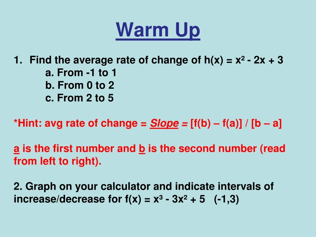
1. Warm Up • Find the average rate of change of h(x) = x² - 2x + 3 • a. From -1 to 1 • b. From 0 to 2 • c. From 2 to 5 • *Hint: avg rate of change = Slope = [f(b) – f(a)] / [b – a] • a is the first number and b is the second number (read from left to right). • 2. Graph on your calculator and indicate intervals of increase/decrease for f(x) = x³ - 3x² + 5 (-1,3)

2. 2.4 Using Linear Models Modeling Real-World Data Predicting with Linear Models (Find Lines of Best Fit – hand drawn and w/graphing calc). Graph linear equations.

3. 1) Modeling Real-World Data Big idea… Use linear equations to create graphs of real-world situations. Then use these graphs and equations to make predictions about past and future trends.

4. 1) Modeling Real-World Data Example 1: There were 174 words typed in 3 minutes. There were 348 words typed in 6 minutes. How many words were typed in 5 minutes?

5. 1) Modeling Real-World Data x = independent y = dependent (x, y) = (time, words typed ) (x1, y1) = (3, 174) (x2, y2) = (6, 348) (x3, y3) = (5, ?) Solution: y = 58x, y = 58(5) total words = 290 400 300 200 100 1 2 3 4 5 6 Time (minutes)

6. 2) Predicting with Linear Models • You can extrapolate with linear models to make predictions based on trends. • Extrapolate - extend (a graph, curve, or range of values) by determining unknown values from trends in the known data.

7. 2) Predicting with Linear Models Example 1: After 5 months the number of subscribers to a newspaper was 5730. After 7 months the number of subscribers was 6022. Write an equation for the function. How many subscribers will there be after 10 months?

8. 2) Predicting with Linear Models (x, y) = (months, subscribers) (x1, y1) = (5, 5730) (x2, y2) = (7, 6022) (x3, y3) = (10, ?) Equation:y = mx + b 8000 6000 4000 2000 2 4 6 8 10 Time (months)

9. 2) Predicting with Linear Models (x, y) = (months, subscribers) (x1, y1) = (5, 5730) (x2, y2) = (7, 6022) (x3, y3) = (10, ?) Equation:y = mx + b 8000 6000 4000 2000 2 4 6 8 10 Time (months)

10. 2) Predicting with Linear Models (x, y) = (months, subscribers) (x1, y1) = (5, 5730) (x2, y2) = (7, 6022) (x3, y3) = (10, ?) Equation:y = mx + b 8000 6000 4000 2000 2 4 6 8 10 Time (months)

11. 2) Predicting with Linear Models (x, y) = (months, subscribers) (x1, y1) = (5, 5730) (x2, y2) = (7, 6022) (x3, y3) = (10, 6460) Equation:y = mx + b y = 146x + 5000 y = 146(10) + 5000 = 6460 Total subscribers = 6460 8000 6000 4000 y-intercept 2000 2 4 6 8 10 Time (months)

12. Scatter Plots • Connect the dots with a trend line (line of best fit) to see if there is a trend in the data.

13. Types of Scatter Plots Strong, positive correlation Weak, positive correlation

14. Types of Scatter Plots Strong, negative correlation Weak, negative correlation

15. Types of Scatter Plots No correlation

16. Scatter Plots Example 1: The data table below shows the relationship between hours spent studying and student grade. • Draw a scatter plot. Decide whether a linear model is reasonable. • Draw a line of best fit. Write the equation for the line.

17. Scatter Plots (x, y) = (hours studying, grade) (3, 65) (1, 35) (5, 90) (4, 74) (1, 45) (6, 87) Equation: y = mx + b 100 90 80 70 60 50 40 30 1 2 3 4 5 6 Hours studying

18. Scatter Plots (x, y) = (hours studying, grade) (3, 65) (1, 35) (5, 90) (4, 74) (1, 45) (6, 87) • Based on the graph, is a linear model reasonable? 100 90 80 70 60 50 40 30 1 2 3 4 5 6 Hours studying

19. Scatter Plots (x, y) = (hours studying, grade) (3, 65) (1, 35) (5, 90) (4, 74) (1, 45) (6, 87) • Equation: y = mx + b y = 10.45x + 31.16 100 90 80 70 60 50 40 30 1 2 3 4 5 6 Hours studying

20. Phone Charges The monthly cost C, in dollars, of a certain cellular phone plan is given by the function C(x) = 0.38x + 5, where x is the number of minutes used on the phone. a.) What is the cost if you talk on the phone for 50 minutes? b.) Suppose your monthly bill is $29.32. How many minutes did you use the phone? C.) Suppose that you budget yourself $60 per month for the phone. What is the maximum number of minutes that you can talk?

21. Phone Charges The monthly cost C, in dollars, of a certain cellular phone plan is given by the function C(x) = 0.38x + 5, where x is the number of minutes used on the phone. a.) What is the cost if you talk on the phone for 50 minutes? C(50) = 0.38 (50) + 5 = $24.00 b.) Suppose your monthly bill is $29.32. How many minutes did you use the phone? 29.32 = 0.38x + 5 x = 64 minutes C.) Suppose that you budget yourself $60 per month for the phone. What is the maximum number of minutes that you can talk? 60 ≥ 0.38x + 6 144.73 ≥ x; x ≤ 144 mins

22. Supply and Demand Suppose the quantity supplied, S, and quantity demanded, D, of cellular telephones each month are given by the following functions, where p is the price(in dollars) of the telephone: S(p) = 60p – 900 and D(p) = -15p + 2850 The equilibrium priceis the price at which S(p) = D(p) a.) Find the equilibrium price. What is the equilibrium quantity, the amount demanded (or supplied), at the equilibrium price? b.) Determine the prices for which quantity supplied is greater than quantity demanded. That is, solve S(p) > D(p) c.) Graph S(p) and D(p) and label the equilibrium price.

23. Supply and Demand Suppose the quantity supplied, S, and quantity demanded, D, of cellular telephones each month are given by the following functions, where p is the price(in dollars) of the telephone: S(p) = 60p – 900 and D(p) = -15p + 2850 The equilibrium priceis the price at which S(p) = D(p) a.) Find the equilibrium price. What is the equilibrium quantity, the amount demanded (or supplied), at the equilibrium price? equilibrium price = $50, S(50) = D(50) = 2100 phones b.) Determine the prices for which quantity supplied is greater than quantity demanded. That is, solve S(p) > D(p) 60p – 900 > -15p + 2850 p > $50 c.) Graph S(p) and D(p) and label the equilibrium price.

24. c.) Graph S(p) and D(p) and label the equilibrium price.

25. Assignment 2.4 #1 p.101 1-10, 11-35 by 4’s