Download

1 / 60
600 likes | 663 Views
This advanced computer science department research delves into fast marching on triangulated domains, level sets, viscosity SFS, and minimal geodesics. It includes a brief historical review and details applications in joint works. The methodology involves upwind schemes, continuous morphology, and weight domains for computing distances efficiently. The text covers numerical approximations, 2D and 3D grids, path planning, acute angle updates, minimal geodesics, Voronoi diagrams, and offsets. It presents edge integration, shape-from-shading techniques, and computational complexities in solving Eikonal equations. The research emphasizes optimal update procedures, consistency, and minimization approaches for geometric processing tasks.

E N D
Computer Science Department • Technion-Israel Institute of Technology Fast Marching on Triangulated Domains Ron Kimmel www.cs.technion.ac.il/~ron • Geometric Image Processing Lab
Brief Historical Review • Upwind schemes: Godunov 59 • Level sets: Osher & Sethian 88 • Viscosity SFS: Rouy & Tourin 92, (Osher & Rudin) • Level sets SFS: Kimmel & Bruckstein 92 • Continuous morphology: Brockett & Maragos 92,Sapiro et al. 93 • Minimal geodesics: Kimmel, Amir & Bruckstein 93 • Fast marching method: Sethian 95 • Fast optimal path: Tsitsiklis 95 • Level sets on triangulated domains:Barth & Sethian 98 • Fast marching on triangulated domains: Kimmel & Sethian 98 • Applications based on joint works with: Elad, Kiryati, Zigelman
1D Distance: Example 1 • Find distance T(x), given T(x0)=0. • Solution: T(x)=|x-x0|. • except at x0. T(x) x x0
Find the distance T(x), given T(x0)=T(x1)=0 Solution: T(x) = min{|x-x0|,|x-x1|}, Again, , except x0,x1and(x0+x1)/2. 1D Distance: Example 2 T(x) x x0 x1
1D Eikonal Equation with boundary conditions T(x0)=T(x1)=0. • Goal: Compute T that satisfies the equation `the best'. T(x) x x0 x1
Numerical Approximation • Restrict , where h= grid spacing. • Possible solutions for are T(x) x x0 x1
Approximation II • Updated i has always • `upwind' from where the `wind blows' T(x) x x0 x1
Update Procedure Set , and T(x0)=T(x1)=0. REPEAT UNTIL convergence, • FOR each i T i T i+1 T i-1 i i-1 i+1 h
Update Order What is the optimal order of updates? Solution I: Scan the line successively left to right. N scans, i.e. O(N ) Solution II: Left to right followed by right to left. Two scans are sufficient. (Danielson`s distance map 1980) Solution III: Start from x0, update its neighboring points, accept updated values, and update their neighbors, etc. 2 1 2 3 1 2
Weighted Domains • Local weight ,Arclength • Goal: distance function characterized by: • By the chain rule: • The Eikonal equation is T(x) F(x) x x0 x1
2D Rectangular Grids Isotropic inhomogeneous domains Weighted arclength: the weight is Goal: Compute the distance T(x,y) from p0 where
Upwind Approximation in 2D T ij T i+1,j T i,j-1 i+1,j T i,j-1 i+1,j T i-1,j ij i,j+1 i-1,j
2D Approximation Initialization: • given initial value or Update: Fitting a tilted plane with gradient , and two values anchored at the relevant neighboring grid points. T 1 i+1,j T 2 i,j-1 ij i,j+1 i-1,j
Computational Complexity • T is systematically constructed from smaller to larger T values. • Update of a heap element is O(log N). • Thus, upper bound of the total is O(N log N). www.math.berkeley.edu/~sethian
Shortest Path on Flat Domains Why do graph search based algorithms (like Dijkstra's) fail?
Edge Integration Cohen-Kimmel, IJCV, 1997. Solve the 2D Eikonal equation given T(p)=0 Minimal geodesic w.r.t.
Shape from Shading Rouy-Tourin SIAM-NU 1992, Kimmel-Bruckstein CVIU 1994, Kimmel-Sethian JMIV 2001. Solve the 2D Eikonal equation where Minimal geodesic w.r.t.
Path Planning 3 DOF Solve the Eikonal Eq. in 3D {x,y,j}-CS given T(x0,y0,j0)=0, Minimal geodesic w.r.t.
Path Planning 4 DOF Solve the Eikonal Eq. in 4D Minimal geodesic w.r.t.
Update Acute Angle Given ABC, update C. Consistency and monotonicity: Update only `from within the triangle' hinABC Find t=EC that satisfies the gradient approximation (t-u)/h= F. c c
Update Procedure We end up with: t must satisfy u<t, and hinABC. The update procedure is IF (u<t) AND (a cos q < b(t-u)/t < a/cosq) THEN T(C) = min {T(C),t+T(A)}; ELSE T(C)=min {T(C),bF+T(A),aF+T(B)}. u C B A
Obtuse Problems This front first meets B, next A, and only then C. A is `supported’ by a single point. The supported section of incoming fronts is a limited section.
Solution by splitting Extend this section and link the vertex to one within the extended section. Recursive unfolding: Unfold until a new vertex Q is found. Initialization step!
Recursive Unfolding: Complexity e = length of longest edge The extended section maximal area is bounded bya<= e /(2a ). The minimal area of any unfolded triangle is bounded below a >= (h a ) q /2, The number of unfolded triangles before Q is found is bounded by m<= a /a = e /(q h a ). max 2 max min 2 min min min min 2 2 3 max max min min min min
1st Order Accuracy The accuracy for acute triangles isO(e ) Accuracy for the obtuse case O(e /(p-q )) max max max
Linear Interpolation ODE ‘back tracking’
Voronoi Diagrams and Offsets • Given n points, { p D, j 0,..,n-1} • Voronoi region: • G = {p D| d(p,p ) < d(p,p ), V j = i}. j i i j
Marching Triangles • The intersection set of two functions is linearly interpolated via `marching triangle'
A frame grabber built at the Technion by Y Grinberg Lego Mindstorms rotates the laser (E. Gordon) Cheap and Fast 3D Scanner • PC + video frame grabber. • Video camera. • Laser line pointer. Joint with G. Zigelman motivated by simple shape from structure light methods, like Bouguet-Perona 99, Klette et al. 98
Examples of Decimation Decimation - 3% of vertices Sub-grid sampling
Texture Mapping • Environment mapping: Blinn, Newell (76). • Environment mapping: Greene, Bier and Sloan (86). • Free-form surfaces: Arad and Elber (97). • Polyhedral surfaces: Floater (96, 98), Levy and Mallet (98). • Multi-dimensional scaling: Schwartz, Shaw and Wolfson (89).
Difficulties • Need for user intervention. • Local and global distortions. • Restrictive boundary conditions. • High computational complexity.
Flattening via MDS • Compute geodesic distances between pairs of points. • Construct a square distance matrix of geodesic distances^2. • Find the coordinates in the plane via multi-dimensional scaling. The simplest is `classical scaling’. • Use the flattened coordinates for texturing the surface, while preserving the texture features. Zigelman, Kimmel, Kiryati, IEEE T. on Visualization and Computer Graphics (in press). 0 0 0