Download
1 / 18
180 likes | 201 Views
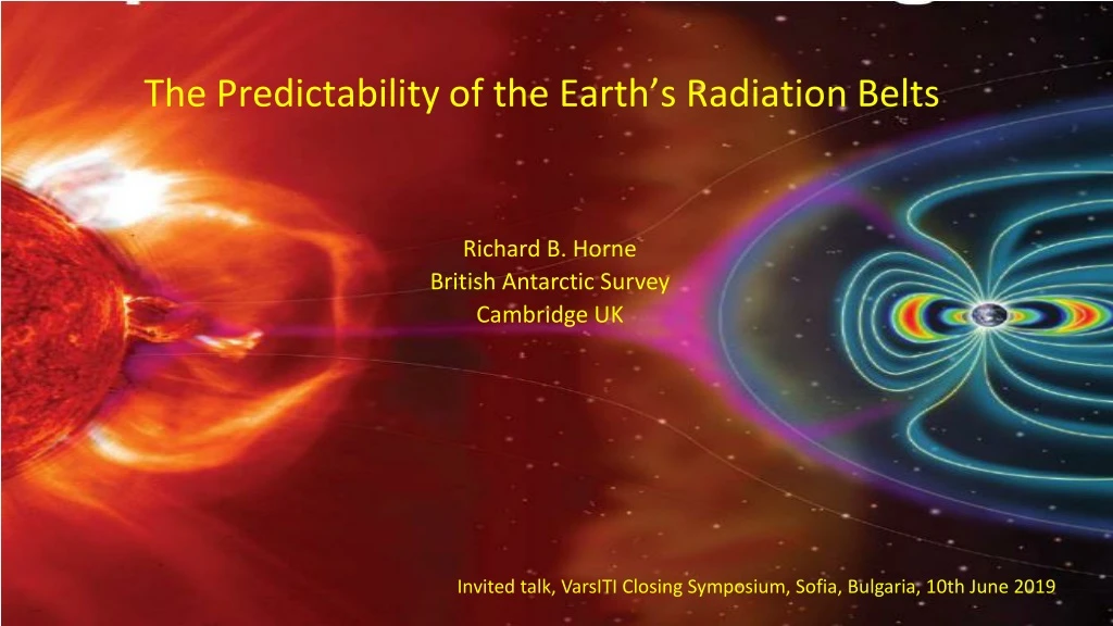
The Predictability of the Earth’s Radiation Belts. Richard B. Horne British Antarctic Survey Cambridge UK. Invited talk, VarsITI Closing Symposium, Sofia, Bulgaria, 10th June 2019. Outline. Why do we need to predict the radiation belts ? The proton belt – an example

E N D
The Predictability of the Earth’s Radiation Belts Richard B. Horne British Antarctic Survey Cambridge UK Invited talk, VarsITI Closing Symposium, Sofia, Bulgaria, 10th June 2019
Outline • Why do we need to predict the radiation belts ? • The proton belt – an example • Variability of the electron belts • Physical processes that control the electron radiation belts • Example forecasting system - SaRIF
Earth’s Radiation Belts • Electrons and ions trapped inside the magnetic field • Only one proton belt • Two electron belts • Energies > 1 MeV • Peaks near 1.6 and 4.5 Re • Outer electron belt highly variable • Hazardous for spacecraft and humans
Solar Energetic Particle Events – Proton Belt • Maybe 1 – 3 per solar cycle • Protons become trapped in the outer region of the proton belt • Last for months – then released in a magnetic storm • O’Hare et al., (2019): • 10Be and 36Cl in ice cores in ~660 BC indicate an event 10 times bigger than we have ever recorded directly (1956 event)
Proton Radiation Belt Before March 1991 After March 1991 SEP event
Proton Belt - Degradation of Satellite Solar Arrays Cover-glass thickness 150 um • Electric propulsion used commercially since 2015 • ~ 200 days to reach orbit Launch before event – lose 3.5% of power before reaching orbit Launch after event – lose 8% of power before reaching orbit Lozinski et al. SW (2019)
Variability of the Electron Belts - 1. Day to Day Geostationary orbit • How do you produce high energy ( >1 MeV) electrons? • What causes the variations? • No electrons greater than ~800 keV in the inner belt
Variability of the Electron Belts – 2. CME/Shock Compression Horne and Pitchford, (2015) • New Electron Belt Formed in 2 Minutes • Slot region ‘filled-in’ • Decay timescale ~ year Geostationary orbit 8,000 km Slot region orbit
Baker et al. Nature (2004) Variability of the Electron Belts – 3. Major Geomagnetic Storms GEO orbit (approx.) • Haloween storms of 23rd Oct to 6th Nov 2003 • 47 satellites reported malfunctions • 1 total loss • 10 satellites – loss of service for more than 1 day • Electrons at much lower L • Decay time ~ year
Variability of the Electron Belts - 4. Rapid Loss Rapid loss – or drop out • Baker et al. [2016]
b). Plasmaspheric hiss Electron Radiation Belt Dynamics a). EMIC waves SC1 Rumba 10-12 2.0 CRRES - FMI Magnetopause inward motion – causes loss rapid motion – acceleration 2.0 102 1.5 10-13 1.5 1.0 V2m-2Hz-1 Frequency (kHz) 1.0 100 Frequency (Hz) nT2Hz-1 10-14 0.5 0.5 0.0 10-15 10-2 0.0 Magnetic field fluctuations driven by ULF waves 13:49:29 13:49:34 13:49:24 13:00 14:00 15:00 Hiss waves Loss UT UT Chorus waves Acceleration and loss EMIC waves Loss > 2 MeV Electron drift path SC1 Rumba 2.0 10-8 10-9 1.5 • Plus other waves and transport processes • Activity, location and energy dependent • Nonlinear, timescale –us to days 10-10 1.0 V2m-2Hz-1 10-11 0.5 10-12 0.0 10-13 13:01:12 13:01:17 13:01:22 UT
Time Dependent Model of the Electron Belts Pitch angle diffusion Energy diffusion Solve the Fokker-Planck Equation Model includes: • Wave-particle interactions • Radial transport • Loss to the atmosphere • Loss to the magnetopause Radial diffusion Loss to atmosphere Loss to the magnetopause
Satellite Risk Prediction and Radiation Forecast (SaRIF) • Solar wind data from L1 • Pressure and IMF Bz • Forecast magnetopause • Forecast Kp • Plasma wave properties scaled by Kp • Calculate pitch angle and energy diffusion coefficients • ULF wave power scaled by Kp • Calculate radial diffusion coefficients • Electron flux and energy spectrum scaled by Kp • Calculate spectrum at outer boundary • Calculate flux at low energy boundary • Solve Fokker-Planck Equation and forecast entire radiation belt flux
Example - 30 year Reconstruction of the Radiation Belts Coronal holes - Fast solar wind Glauert et al., SW, (2018) GEO Slot Inner belt
Satellite Risk Prediction and Radiation Forecast (SaRIF) – Geostationary Orbit Available as SaRIF via the ESA Space Weather Web portal
Satellite Risk Prediction and Radiation Forecast (SaRIF) – Geostationary Orbit Available as SaRIF via the ESA Space Weather Web portal
Predictability - Timescales • Sun to L1 – usually 1-2 days, but the fastest is 14.5 hours • L1 to magnetopause - ~ 30 minutes, but can be much faster • Magnetopause to radiation belts – from tens of minutes to a few hours • Inside the magnetosphere: • Plasma waves can cause acceleration to MeV energies and loss – from milliseconds to days • Transport across the magnetic field - from hours to days • Magnetopause compression can cause rapid loss ~ tens of minutes – and or acceleration • Substorm cycle – few hours – but can repeat for days - storms • If the solar wind is ‘quiet’ we may be able to forecast up to 24 hours, maybe more – but rapid changes in the solar wind can reduce or remove our ability to predict • Essential to know solar wind pressure and IMF Bz
Summary • Electron radiation belts can vary on timescales from few minutes to days • To predict – need forecast of solar wind at L1 – pressure, IMF Bz • We must also develop more understanding of: • Non-linear wave-particle interactions on timescales from milliseconds to days • Diffusive and non-diffusive transport • Shock driven compression of the magnetopause • Magnetic field disruptions during storms • Changes in the source electrons • These are major challenges • But they are needed to protect satellites from Space Weather