Download

1 / 38
420 likes | 909 Views
Fourier Transform. A periodic function may be decomposed as the sum of sines and cosines of varying amplitudes and frequencies. One-dimensional Discrete Fourier Transform. Suppose f=[f 0 ,f 1 ,f 2 , … ,f n-1 ] is a sequence of length N

E N D
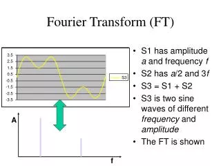
A periodic function may be decomposed as the sum of sines and cosines of varying amplitudes and frequencies.
One-dimensional Discrete Fourier Transform • Suppose f=[f0,f1,f2,…,fn-1] is a sequence of length N • We define its DFT to be the sequence F=[F0,F1,F2,…,Fn-1] • Where
This definition can be expressed as a matrix multiplication: • F=Ff • Where F is an N x N matrix defined by
The inverse DFT is very similar to the forward transform: • We can express this as a matrix product: • f=F-1F
The properties of one-dimensional DFT • Linearity • Shifting • Conjugate symmetry • Convolution
Linearity • Suppose f and g are two vectors of equal length, and p and q are scalar, with h=p f +q g. • If F,G, and H are the DFT of f, g, and h, we have H = p F + q G • This follows from the definitions of • F=Ff, G=Fg, H=Fh
Multiply (-1)n DFT DFT X X’ X’ is equal to x with the swapping of the left and right halves (p150) Shifting • Suppose x={x1,x2,x3,…,xk} • xn X’
Conjugate symmetry • X is real of length N, then its DFT satisfies the condition that • Xk= XN-k for all k=1,2,3,…,N-1 • Thus x1= x7 , x2= x6 , x3= x5, x4= x4, which means x4 must be real
Convolution(1) • Suppose x and y are two vectors of the same length N. We define their convolution to be the vector • z=x*y (commutative x*y=y*x) • Where • If N=4, then • Z0=(x0y0+x1y-1+x2y-2+x3y-3)/4
Convolution(2) • …y0 y1 y2 y3 y0 y1 y2 y3… =…y0 y-3 y-2 y-1 y0 y1 y2 y3… • Convolution theorem • Z,X and Y are the DFT of z=x*y, x and y, respectively, then Z=X.Y • It provides us with another way of performing convolution: multiply the DFT’s of our two vectors and invert the result
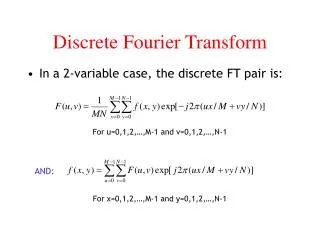
Two-dimensional DFT • The forward and inverse transforms for an MxN matrix
Properties of the 2D Fourier Transform • Similarity • The DFT as a spatial filter • Separability • Linearity • The convolution theorem • The dc coefficient • Shifting • Conjugate symmetry • Displaying transforms
Similarity • The forward and inverse transforms are very similar with the exception of the scale factor 1/MN in the inverse transform and the negative sign in the exponent of the forward transform
The DFT as a spatial filter • are independent of the values f or F • It means that every value F(u,v) is obtained by multiplying every value of f(x,y) by a fixed value and adding up all the results. This is what a linear spatial filter does.
Only depends on x and u, and is independent of y and v This means we can break down our formula above to simpler one that works on single rows or columns Separability
The convolution theorem(1) • convolve an image M with a spatial filter SM*S • Slow if S is large • The convolution theorem states that this can be done by the following steps: • Pad S with zeroes S’ (S’ is the same size as M) • Perform F(M) and F(S’) • form the element-by-element product of these two transforms: F(M).F(S’) • take the inverse transform of the result: F-1(F(M).F(S’))
The dc coefficient • The value F(0,0) is called the DC coefficient • Put u=0,v=0 in the forward DFT, then • F(0,0) is the sum of all f(x,y)
DC coefficient Shifting • For purpose of display, it is convenient to have the DC coefficient in the center. This can be done by multiplying f(x,y) by (-1)x+y before performing the DFT
Conjugate symmetry • If we make the substitutions u=-u and v=-v , then • F(u,v)=F*(-u+pM,-v+qN) for any integers p and q.
Displaying transforms • F(u,v) are complex numbers • Two approach: 1. Use imshow to view |F(u,v)| /DC coefficient 2. Use mat2gray to view |F(u,v)| directly. Problem: DC is larger than all other values and thus will result in a single white dot surrounded by black Solution: take Log(1+ |F(u,v)|)
Filtering in the frequency domain • Ideal filtering • Butterworth filtering • Gaussian filtering • Homomorphic filtering
Ideal filtering (Low-pass filtering) • Observation: In the frequency domain, the low frequency components are toward the center • criterion: multiply the transform by a matrix in such a way that center values are maintained and values away from the center are either removed or minimized.
With D=15 Ideal filtering (Low-pass filtering) • Ideal low-pass matrix • m(x,y)=
ringing effect With D=15 Ideal filtering (High-pass filtering) • High-pass filtering • m(x,y)=
Butterworth Filtering • Low-pass filter f(x)=1/(1+(x/D)2n) • High-pass filter f(x)=1/(1+(D/x)2n) n=2 n=4 n=4 n=2
Low-pass filtering High-pass filtering
Gaussian Filtering (low-pass filter) • f(x)=e-x^2/2σ^2
Gaussian filters are important for a number of reasons: 1. they are mathematically very well behaved; in particular, the Fourier transform of a Gaussian filter is another Gaussian 2. they are rotationally symmetric, so are very good starting points for some edge-detection algorithms 3. they are separable (apply it on rows first and then on columns) 4. the convolution of two Gaussians is another Gaussian
σ=30 σ=10
Gaussian Filtering (high-pass filter) Gaussian high-pass filter=1-gaussian low-pass filter σ=10 σ=30
Homomorphic filtering • f(x,y)=i(x,y)·r(x,y) i(x,y): illumination r(x,y): reflectance 0<i(x,y)<infinite 0<r(x,y)<1 • log f(x,y)=log i(x,y) + log r(x,y)
image i(x,y) r(x,y) sum exp output Low-pass filtering high-pass filtering log
Problem: Given a value log f(x,y), we can not determine the values of log i(x,y) and log r(x,y). • Solution: Use high-boost filter of Fourier transform
image FFT FFT-1 exp output log High-boost filtering
By trial and error to produce bands of suitable width and on such places as to obscure detail in our image y=0.5 + 0.4 sin x 0.1<= y <=1.0