MRP

1. MRP

2. Learning Objectives • Describe the conditions under which MRP is most appropriate. • Describe the inputs, outputs, and nature of MRP processing. • Explain how requirements in a master production schedule are translated into material requirements for lower-level items. • Discuss the benefits and requirements of MRP.

3. Learning Objectives • Explain how an MRP system is useful in capacity requirements planning. • Outline the potential benefits and some of the difficulties users have encountered with MRP. • Describe MRP II and its benefits. • Describe ERP, what it provides, and its hidden costs.

4. MRP • Time-phase based • Subassemblies • Components • Raw materials End products MRP • Material requirements planning (MRP): Computer-based information system that translates master schedule requirements for end items into time-phased requirements for subassemblies, components, and raw materials.

5. Independent and Dependent Demand Independent Demand Dependent Demand A C(2) B(4) D(2) E(1) D(3) F(2) Independent demand is uncertain. Dependent demand is certain.

6. Dependant Demand • Dependent demand: Demand for items that are subassemblies or component parts to be used in production of finished goods. • Once the independent demand is known, the dependent demand can be determined.

7. Demand “Lumpy” demand Demand Stable demand Demand Time Time Amount on hand Amount on hand Safety stock Time Time

8. Overview of MRP MRP Inputs MRP Processing MRP Outputs Changes Order releases Master schedule Planned-order schedules Primary reports Exception reports Bill of materials Planning reports MRP computer programs Secondary reports Performance- control reports Inventory records Inventory transaction

9. MPR Inputs • Master Production Schedule • Time-phased plan specifying timing and quantity of production for each end item. • Material Requirement Planning Process Product Structure Tree Inventory Lead Times

10. Master Schedule Master schedule: One of three primary inputs in MRP; states which end items are to be produced, when these are needed, and in what quantities. Cumulative lead time: The sum of the lead times that sequential phases of a process require, from ordering of parts or raw materials to completion of final assembly.

11. Planning Horizon Assembly Subassembly Fabrication Procurement 6 7 1 2 3 4 5 8 9 10 Time Period (weeks)

12. Bill-of-Materials Bill of materials (BOM):One of the three primary inputs of MRP; a listing of all of the raw materials, parts, subassemblies, and assemblies needed to produce one unit of a product. Product structure tree: Visual depiction of the requirements in a bill of materials, where all components are listed by levels. Low-level coding: Restructuring the bill of materials so that multiple occurrences of a component all coincide with the lowest level the component occurs

13. Product Structure Tree Level 0 Chair Leg Assembly Back Assembly 1 Seat Cross bar Side Rails (2) Cross bar Back Supports (3) Legs (2) 2 E (4) E (4) E E (2) Level 0 1 2 3

14. Inventory Records • One of the three primary inputs in MRP • Includes information on the status of each item by time period • Gross requirements • Scheduled receipts • Amount on hand • Lead times • Lot sizes • And more …

15. Inventory Requirements • Net requirements: • Available Inventory: Net Requirements = Gross Requirements – Available Inventory Available Inventory = Projected on hand – Safety stock – Inventory allocated to other items

16. Assembly Time Chart Procurement of raw material D Fabrication of part E Subassembly A Procurement of raw material F Final assembly and inspection Procurement of part C Procurement of part H Subassembly B Fabrication of part G Procurement of raw material I 6 7 1 2 3 4 5 8 9 10 11

17. Time-Phased Product Structure Must have D and E completed here so production can begin on B Start production of D 1 week A B C D E F G 1 2 1 1 2 3 2 weeks weeks weeks weeks weeks weeks weeks D (2) 2 weeks E (2) A 2 weeks 1 week 2 weeks G (1) 3 weeks F (2) 1 week D (2) | | | | | | | | 1 2 3 4 5 6 7 8 Time in weeks Lead time 2 weeks to produce B (2) E (2) 1 week C (3)

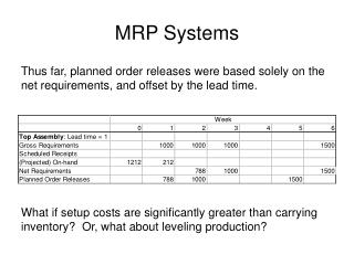
18. Gross Requirements Plan Week 1 2 3 4 5 6 7 8 Lead Time Required date 50Order release date 50 1 week Required date 100Order release date 100 2 weeks Required date 150Order release date 150 1 week Required date 200 300Order release date 200 300 2 week Required date 300Order release date 300 3 weeks Required date 600 200Order release date 600 200 1 week Required date 300Order release date 300 2 week

19. Net Requirements Plan

20. Net Requirements Plan

21. MRP Processing • Gross requirements • Schedule receipts • Projected on hand • Net requirements • Planned-order receipts • Planned-order releases

22. MPR Processing • Gross requirements • Total expected demand • Scheduled receipts • Open orders scheduled to arrive • Projected on hand • Expected inventory on hand at the beginning of each time period

23. MPR Processing • Net requirements • Actual amount needed in each time period • Planned-order receipts • Quantity expected to be received at the beginning of the period • Offset by lead time • Planned-order releases • Planned amount to order in each time period

24. Lot-Sizing Techniques • Lot-for-lot techniques order just what is required for production based on net requirements • May not always be feasible • If setup costs are high, costs may be high as well • Economic order quantity (EOQ) • EOQ expects a known constant demand and MRP systems often deal with unknown and variable demand

25. Lot-Sizing Techniques • Part Period Balancing (PPB) looks at future orders to determine most economic lot size • EPP = setup cost / holding cost • Programming technique • Assumes a finite time horizon • Effective, but computationally burdensome

26. Lot-for-Lot Example Holding cost = $1/week; Setup cost = $100/times; Lead time = 1 week

27. Lot-for-Lot Example No on-hand inventory is carried through the system Total holding cost = $0 There are seven setups for this item in this plan Total setup cost = 7 x $100 = $700 Holding cost = $1/week; Setup cost = $100/times; Lead time = 1 week

28. EOQ Lot Size Example Holding cost = $1/week; Setup cost = $100/times; Lead time = 1 week Average weekly gross requirements = 27; EOQ = 73 units

29. EOQ Lot Size Example Annual demand = 1,404 Total cost = setup cost + holding cost Total cost = (1,404/73) x $100 + (73/2) x ($1 x 52 weeks) Total cost = $3,798 /year Cost for 10 weeks = $3,798 x (10/52) = $730 Or Total cost = setup cost + holding cost Total cost = 4 x $100 + 318 x ($1 /weeks) Total cost = $718 Holding cost = $1/week; Setup cost = $100/times; Lead time = 1 week Average weekly gross requirements = 27; EOQ = 73 units

30. PPB Example Holding cost = $1/week; Setup cost = $100; Lead time = 1 week ; EPP = 100 units

31. PPB Example Trial Lot Size Periods (cumulative net Costs Combined requirements) Part Periods Setup Holding Total 2 30 0 2, 3 70 40 = 40 x 1 2, 3, 4 70 40 = 40 x 1 2, 3, 4, 5 80 70 = 50 x 1 + 10 x 2 100 70 170 2, 3, 4, 5, 6 120 230 = 90 x 1 + 50 x 2 + 40 x 1 + + + + = = = = Combine periods 2 - 5 as this results in the Part Period closest to the EPP 6 40 0 6, 7 70 30 = 30 x 1 6, 7, 8 70 30 = 30 x 1 6, 7, 8, 9 100 120 = 60 x 1 + 30 x 2 100 120 220 Combine periods 6 - 9 as this results in the Part Period closest to the EPP 10 55 0 100 0 100 Total cost 300 190 490 Holding cost = $1/week; Setup cost = $100; EPP = 100 units

32. Lot-Sizing Summary Lot-for-lot $700 EOQ $730 PPB $490 For these three examples Wagner-Whitin would have yielded a plan with a total cost of $455 for this example

33. Example Holding cost = $1/week; Setup cost = $100; Lead time = 1 week ; EPP = 100 units

34. Lot-Sizing Summary • In theory, lot sizes should be recomputed whenever there is a lot size or order quantity change • In practice, this results in system nervousness and instability • Lot-for-lot should be used whenever economical • Lot sizes can be modified to allow for scrap, process constraints, and purchase lots

35. Lot-Sizing Summary • Use lot-sizing with care as it can cause considerable distortion of requirements at lower levels of the BOM • When setup costs are significant and demand is reasonably smooth, PPB, Wagner-Whitin, or EOQ should give reasonable results

36. Updating the System • Regenerative system • Updates MRP records periodically • Net-change system • Updates MPR records continuously

37. MRP Primary Reports • Planned orders - schedule indicating the amount and timing of future orders. • Order releases - Authorization for the execution of planned orders. • Changes - revisions of due dates or order quantities, or cancellations of orders.

38. MRP Secondary Reports • Performance-control reports system evaluation, deviation, late delivery, stockouts • Planning reports useful for forecasting future inventory, assess future material requirement • Exception reports late or overdue orders, excessive scrap rate, requirement of non-existing parts

39. Material Checking & Balancing • Use for monitoring of amount of part and product during processes • Needs information to balance materials • Accumulative production planning or target plan • BOM or Assembly diagram • Normally periodic checked

40. Material Checking & Balancing G C B D I K J H E A F Week 9 8 7 6 5 4 3 2 1 0 Balancing chart Target Plan Accumulative production J F M A M J J A S O N D A B C D E F G H I J K Assembly diagram

41. Resource Requirements Profile 200 – 150 – 100 – 50 – – 200 – 150 – 100 – 50 – – Capacity exceeded in periods 4 & 6 Lot 6 “split” Lot 11 moved Available capacity Available capacity Lot 11 Lot 6 Lot 6 Lot 11 Standard labor hours Standard labor hours Lot 9 Lot 9 Lot 15 Lot 15 Lot 12 Lot 12 Lot 7 Lot 7 Lot 2 Lot 2 Lot 4 Lot 4 Lot 1 Lot 1 Lot 10 Lot 10 Lot 14 Lot 14 Lot 16 Lot 16 Lot 13 Lot 13 Lot 8 Lot 8 Lot 3 Lot 3 Lot 5 Lot 5 1 1 2 2 3 3 4 4 5 5 6 6 7 7 8 8 Period (a) Period (b)

42. Smoothing Tactics • Overlapping • Sends part of the work to following operations before the entire lot is complete • Reduces lead time • Operations splitting • Sends the lot to two different machines for the same operation • Shorter throughput time but increased setup costs • Lot splitting • Breaking up the order into smaller lots and running part ahead of schedule

43. Other Considerations • Safety Stock • Lot sizing • Lot-for-lot ordering • Economic order quantity • Fixed-period ordering

44. MRP in Services • Food catering service • End item => catered food • Dependent demand => ingredients for each recipe, i.e. bill of materials

45. Benefits of MRP • Low levels of in-process inventories • Ability to track material requirements • Ability to evaluate capacity requirements • Means of allocating production time • Ability to easily determine inventory usage by backflushing • Backflushing: Exploding an end item’s bill of materials to determine the quantities of the components that were used to make the item.

46. Requirements of MRP • Computer and necessary software • Accurate and up-to-date • Master schedules • Bills of materials • Inventory records • Integrity of data

47. MRP II • Expanded MRP with emphasis placed on integration • Financial planning • Marketing • Engineering • Purchasing • Manufacturing

48. MRP II Master production schedule Market Demand Finance Manufacturing Marketing Production plan MRP Adjust master schedule Rough-cut capacity planning Capacity planning Adjust production plan No Yes Requirements schedules No Yes Problems? Problems?

49. ERP • Enterprise resource planning (ERP): • Next step in an evolution that began with MPR and evolved into MRPII • Integration of financial, manufacturing, and human resources on a single computer system.

50. ERP Software • ERP software provides a system to capture and make data available in real time to decision makers and other users in the organization • Provides tools for planning and monitoring various business processes • Includes • Production planning and scheduling • Inventory management • Product costing • Distribution