Download
1 / 48
600 likes | 876 Views
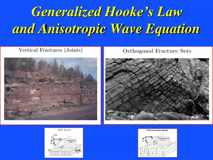
Generalized Hooke’s Law and Anisotropic Wave Equation. Outline. Generalized Hooke’s Law Hooke+Newton =Anisotropic Wave Equation Isotropic Wave Equation P and S waves Summary Appendix. Cards are normal stiffer along 11 direction so stiffness c 11 > c 33. x3. x3. x1. x1.

E N D
Outline • Generalized Hooke’s Law • Hooke+Newton =Anisotropic Wave Equation • Isotropic Wave Equation • P and S waves • Summary • Appendix
Cards are normal stiffer along 11 direction so stiffness c11 > c33 x3 x3 x1 x1 Generalized Hooke’s Law x2 x2 so t11 = c11 e11 andt33= c33 e33 Normal deformation along 11 depends on 11 and 33 stiffnesses (Note buckled cards cause 33 stiff ness weak): so t11 = c11 e11 + c13e33 + c12e22 + c1?e21 Not enough indices for cij What happens if we stress cards along horizontal? How about cijkl ? Any stress induces any strain combination
Stiffness of rock depends on contact plane orientation and component of traction we impose; every type of deformation results along all three different planes. Generalized Hooke’s Law Strain tensor Stress tensor t = c e ij ijkl kl t22 t33 Strains along k face Einstein notation (repeated indicies are summed) Stress along i face t11
Generalized Hooke’s Law (Cauchy in 1800s figured this out) Strain tensor Stress tensor t = c e ij ijkl kl Stiffness tensor 81 constants (3x3x3x3=81) but 21 are independent constants. c ijkl e = e 1). Symmetry of strain: 81->54 kl lk t = t 2). Symmetry of stress: 54->36 kl lk 3). Symmetry of strain energy: 36->21 e Interchange ijwith klbecause kl and ij are dummy variables under summation e t e c e c e W = 0.5 0.5 0.5 = = ij ij ijkl kl klij kl ijij
Symmetry Strain: 81->54 (Cauchy in 1800s figured this out) e kl Strain tensor Stress tensor 9x9 matrix Cmn: 81 independent coefficents. We will show strain symmetry implies Cmn has m=1...9 & n=1...6 indep. values 9x9 matrix: 9+8+7+6+5+4+3+2+1=54 independent values per row t = c e Map ijm 111 22>>2 333 124 135 216 23—7 318 329 ij ijkl kl Stiffness tensor e = e 81->54 1). Symmetry of strain: c kl lk t = c e = c e ijkl ij ijkl ijlk kl lk subtracting both sides gives 0 = (c cijklCmn - c )e ijkl ijlk kl ij has 9 and kl only has 6 independent valuesCmn only has 54 independent comp. Therefore c = c 81->54 ijlk ijkl
Symmetry Stress: 54->36 (Cauchy in 1800s figured this out) t = c e ij ijkl kl Map ijm 111 22>>2 333 124 135 216 23—7 318 329 = c e jikl kl (t = t ) ij ji Subtracting above gives 0 = (c - c )e c = c kl ijkl ijkl jikl jikl cijklCmn ij now has 6 and kl only has 6 independent values Cmn only has 36 indep. components
Energy : 36->21 (Cauchy in 1800s figured this out) Interchange ijwith klbecause kl and ij are dummy variables under summation 3). Symmetry of strain energy: 36->21 e e t e c e c e W = 0.5 0.5 0.5 = = Subtracting above gives ij ij ijkl kl klij kl ijij Cnm=Cmn 6x6 matrix 6x6 c = c cijklCmn 6x6 matrix 36->21 klij ijkl
Generalized Hooke’s Law (Cauchy in 1800s figured this out) Strain tensor Stress tensor t = c e ij ijkl kl Stiffness tensor 81 constants (3x3x3x3=81) but 21 are independent constants Isotropic assumption (rotational symmetry) t = ld e 2me + ij ij kk ij
Isotropic Hooke’s Law (Cauchy in 1800s figured this out) dx m and l not dependent on whether we impress stress on x face, y face, or z face Change in volume normal stress dx t = ld e + 2me Isotropic rock coefficient m shouldn’t depend on orientation of face…..same resistance no matter which face we strain yy yy yy kk t = ld e + 2me t = 2me t = 2me t = 2me shear stress yz xy zz xz zz zz kk yz xy xz Isotropic assumption (rotational symmetry) t = ld e + 2me xx xx kk xx No volume change, only shape change: du/dx=dv/dy=dw/dz=0 t = ld e 2me + ij ij kk ij dx
Isotropic Hooke’s Law (Cauchy in 1800s figured this out) dx m and l not dependent on whether we impress normal stress on x face, y face, or z face Change in volume normal stress dx m and l not dependent on ij t = ld e + 2me yy yy yy kk t = ld e + 2me zz zz zz kk Isotropic assumption (rotational symmetry) t = ld e + 2me ekk = exx + eyy + ezz xx xx kk xx t = ld e 2me + ij ij kk ij Note: dij means we turn off volume changes wheninot equal to j
Why is there a greater stiffness (l+2m) for exx than for the stiffness 2m of eyy and ezz? txx = (l+2m)exx+ leyy + lezz squish coeff. squirt coeff. squirt coeff. squirt Easier to squirt out than to Squish because it squirts out both top+bottom ..thus, stiffer squish coeff. l+2m > l Isotropic assumption (rotational symmetry) t = ld e 2me squish squish + ij ij kk ij squirt
36 components cijkl can be reassembled into a 6x6 matrix Cmn kl Voight Notation 11 22 33 32 13 12
Isotropic (2 parameters) Cubic Symmetry (3 param.) VTI Symmetry (5 param.) 11 Orthotropy (9 param.) 22 33 32 13 12
Outline • Generalized Hooke’s Law • Hooke+Newton =Anisotropic Wave Equation • Isotropic Wave Equation • P and S Waves • Summary • Appendix
c c c c c c ½(c ½(c ½(c u ) u u ) u ) u u u u u + + + = = = ijkl l,kj ijkl ijlk k,lj k,lj k,lj k,lj k,lj k,lj k,lj k,lj ijkl ijkl ijkl ijkl ijkl ijkl (u + u ) k,l l,k Anisotropic Wave Equation in Homogeneous Medium 9 unknowns: u1, u2, u3, t11, t22, t33, t12, t13, t23 t = c e /2 Hooke’s Law 6 indep. eqs. ij,j ij ijkl (1a) k,lj kl l,kj Take derivative of (1a) w/r to xj (assume homogeneous medium) Newton’s Law 3 indep. eqs. (1b) .. .. t u u + F + F r r u = = Substitute (1b) into (1a) yields i i ij,j k,lj i i c 3 indep. eqs. (1c) ijkl 3 unknowns Similar to 1st-order acoustic eqns of Hookes+Newton’s laws we reduced Two elastic 1st-order systems to 1 system with 2nd-order spatial derivatives, i.e. elastic wave equation
Outline • Generalized Hooke’s Law • Hooke+Newton =Anisotropic Wave Equation • Isotropic Wave Equation • P and S waves • Summary • Appendix
(u + u ) k,l l,k Elastic Isotropic Wave Equation in Inhomogeneous Medium Isotropic Hooke’s Coefficients (2a) t = c /2 (2b) General Hooke’s Law ijkl ij c = ldijdkl + m(d ikdjl+ dildjk) (2c) Substitute (2a) into (2b) to get ijkl .. r u + F u u + u )] = [ld + m ( t = l d e + 2 me Substitute (2c) into W.E. (1b) to get i k,k i i,j j,i ij j ij ij ij kk u u (u + u + u ) + u ) +m ( l + m l ,i ,j k,k k,ki i,jj j,ij i,j j,i .. r u + F = (2d) i i or
Elastic Isotropic Wave Equation in homogeneous Medium u u (u + u + u ) + u ) +m ( + m l l ,i ,j k,k k,ki i,jj j,ij i,j j,i .. r u + F = (2d) i i .. u u + F u r + u ) +m ( = l (2e) k,ki i,jj j,ij i i .. 2 (l+m) u + m u u = D D D + F r (2f) 2 u = u - x xu .. D D D D D (l+2m) u - m u u r = D D D D + F (2g) x x Assume homogeneous medium Explicit vector notation
Outline • Generalized Hooke’s Law • Hooke+Newton =Anisotropic Wave Equation • Isotropic Wave Equation • P and S Waves • Summary • Appendix
Decomposition u into scalar and vector potentials Displacement u = Sum of Potentials: Helmholtz_decomposition http://en.wikipedia.org/wiki/Helmholtz_decomposition Motion parallel to k Motion perpendicular to k http://en.wikipedia.org/wiki/Conservative_vector_field ( ) + ) ( Pure P-wave Equation Pure S-wave Equation
Pure P Pure P and S Wave Equations .. (l+2m) u - m u u r = D D D D + F (2g) x x .. 2 (l+2m) r = D F F (2h) u F = D where ik r Plane P wave e propagates in k direction with particlemotion parallel to propagation direction with propagation velocity F ik r ik r = e e D D l+2m r = ik
Compressional Wave (P-Wave) Animation Deformation propagates. Particle motion consists of alternating compression and dilation. Particle motion is parallel to the direction of propagation (longitudinal). Material returns to its original shape after wave passes.
Pure P and S Wave Equations S z .. (l+2m) u - m u u r = D D D D + F x (2g) x x y .. 2 y y m r = D (2i) xy u D = where ik r Plane S wave e propagates in k direction with particle motion perpendicular to propagation direction with propagation velocity m r
Pure SV and SH Plane Waves We relate solution to that of a Shear wave because it only depends on shear strength modulus .. 2 y y z m r = D (2i) x y u= ikx Try plane wave propagating in x direction: (x) = e i Y i j k 0 u d/dx d/dy d/dz xy x Y 0 = = = D D ikx e 0 0 0 Particle motion is not parallel to propagation direction for a S wave Particle motion parallel to propagation direction is not possible for a S plane wave in an isotropic medium
Pure SV and SH Plane Waves .. 2 y y z m r = D (2i) x y u= ikx y Try plane wave propagating in x direction such that (x) = e j i j k 0 u d/dx d/dy d/dz xy x Y = 0 = = D D ikx ikx e 0 0 ike Particle motion is || to vertical & perpendicular to propagation direction for a SV wave. Only true with a plane wave and a 2D medium (no variation of velocity in y-direction) SV m r
Pure SV and SH Plane Waves .. 2 y y z m r = D (2i) x y = where ikx y Try plane wave propagating in x direction such that: (x) = e k i j k 0 d/dx d/dy d/dz y x u x u ikx = ike Y = = D D ikx e 0 0 0 Particle motion is horizontal&perpendicular to propagation direction for a SH wave SH m r
Shear Wave (SV-Wave) Animation z x y Deformation propagates. Particle motion consists of alternating transverse motion. Particle motion is perpendicular to the direction of propagation (transverse). Transverse particle motion shown here is vertical but can be in any direction. However, Earth’s layers tend to cause mostly vertical (SV; in the vertical plane) or horizontal (SH) shear motions. Material returns to its original shape after wave passes.
Love Wave (L-Wave) Animation Deformation propagates. Particle motion consists of alternating transverse motions. Particle motion is horizontal and perpendicular to the direction of propagation (transverse). To aid in seeing that the particle motion is purely horizontal, focus on the Y axis (red line) as the wave propagates through it. Amplitude decreases with depth. Material returns to its original shape after wave passes.
K+4/3m = V r p No volumetric strain P and S Waves “see” Different Things Compression Extension • K = bulk modulus: depends on fluids (low in gas) • m = shear modulus: no contribution from fluid/gas • = density Shear waves can also be polarized
SH Wave Practical Uses 1. Near surface SH refraction -> VSH(z) VSH(z) (m/s) predicted 2. Earthquake studies: S body waves and Love waves observed Harbor fill Resonance S. America earthquake epicenters Cross-section of earth 3-component seismograms Polarization diagrams P-wave Polariz.
Outline • Generalized Hooke’s Law • Hooke+Newton =Anisotropic Wave Equation • Isotropic Wave Equation • P and S Waves • Summary • Appendix
(u + u ) k,l l,k 1. Shear Strain: 2. Anisotropic Wave Equation Summary ij,j k,lj t = c e l,kj /2 Hooke’s Law 6 indep. eqs. ij ijkl (1a) kl Newton’s Law 3 indep. eqs. (1b) .. .. t u u + F + F r r u = = 3. Isotropic Wave Equation (homogeneous) i i ij,j k,lj i i c 3 indep. eqs. ijkl 3 unknowns .. (l+2m) u - m u u r = D D D D + F x x
Direction prop. Direction prop. Direction prop. Love surface wave (free surface) P body wave S body wave (SV or SH or S) Summary 4. P and S Waves “see” Different Things • K = bulk modulus: depends on fluids (low in gas) • m = shear modulus: no contribution from fluid/gas • = density 5. Earthquakes rich in shear, explosions rich in compressional
2D modeling is for a line source and no variation of earth parameters in one of coordinates z x y Summary Line source creates an expanding cylinder, which increases area by r, so geometric spreading is 1/sqrt(r). This is what your 2D acoustic and elastic codes compute; also a tail and a pi/4 phase shift. 3D wave equation 2 2 2 2 2 2 2 dP/dx + dP/dy + dP/dz = (1/c )dP/dt +f 2 2 2 2 2 2 dP/dx + dP/dz = (1/c )dP/dt +f 2 2 2 Line source f(x,z) and 2D medium
2D modeling is for a line source and no variation of earth parameters in one of coordinates z x y Summary Line source creates an expanding cylinder, which increases area by r, so geometric spreading is 1/sqrt(r). This is what your 2D acoustic and elastic codes compute; also a tail and a pi/4 phase shift. 3D wave equation 2 2 2 2 2 2 2 dP/dx + dP/dy + dP/dz = (1/c )dP/dt +f 2 2 2 2 2 2 dP/dx + dP/dz = (1/c )dP/dt +f 2 2 2 Line source f(x,z) and 2D medium
Compliance (or flexibility) matrix…larger values of Sij lead to more felxible materials where small stress leads to large strain
Can a shear stress induce a normal strain?
An orthotropic material has three mutually orthogonal twofold axes of rotational symmetry so that its material properties are, in general, different along each axis. No shear stress Contribution to Normal strain
No yx or yz shear stress contribution to xz shear strain