Download

1 / 42
2.86k likes | 7.81k Views
TWO DEGREE OF FREEDOM SYSTEM. INTRODUCTION. Systems that require two independent coordinates to describe their motion; Two masses in the system X two possible types of motion of each mass. Example: motor pump system.

E N D
INTRODUCTION • Systems that require two independent coordinates to describe their motion; • Two masses in the system X two possible types of motion of each mass. • Example: motor pump system. • There are two equations of motion for a 2DOF system, one for each mass (more precisely, for each DOF). • They are generally in the form of couple differential equation that is, each equation involves all the coordinates.
Equation of motion for forced vibration • Consider a viscously damped two degree of freedom spring-mass system, shown in Fig.5.3. Figure 5.3: A two degree of freedom spring-mass-damper system
Equations of Motion for Forced Vibration The application of Newton’s second law of motion to each of the masses gives the equations of motion: Both equations can be written in matrix form as where [m], [c], and [k] are called the mass, damping, and stiffness matrices, respectively, and are given by
Equations of Motion for Forced Vibration And the displacement and force vectors are given respectively: It can be seen that the matrices [m], [c], and [k] are all 2 x 2 matrices whose elements are known masses, damping coefficient and stiffnesses of the system, respectively.
Equations of Motion for Forced Vibration • Further, these matrices can be seen to be symmetric, so that, where the superscript T denotes the transpose of the matrix. • The solution of Eqs.(5.1) and (5.2) involves four constants of integration (two for each equation). Usually the initial displacements and velocities of the two masses are specified as x1(t = 0) = x1(0) and 1( t = 0) = 1(0), x2(t = 0) = x2(0) and 2 (t = 0) = 2(0).
Free Vibration Analysis of an UndampedSystem By setting F1(t) = F2(t) = 0, and damping disregarded, i.e., c1 = c2 = c3 = 0, and the equation of motion is reduced to: Assuming that it is possible to have harmonic motion of m1 and m2 at the same frequency ωand the same phase angle Φ, we take the solutions as
Free Vibration Analysis of an UndampedSystem Substituting into Eqs.(5.4) and (5.5), Since Eq.(5.7)must be satisfied for all values of the time t, the terms between brackets must be zero. Thus,
Free Vibration Analysis of an UndampedSystem which represent two simultaneous homogenous algebraic equations in the unknown X1 and X2. For trivial solution, i.e., X1 = X2 = 0, there is no solution. For a nontrivial solution, the determinant of the coefficients of X1 and X2 must be zero: or
Free Vibration Analysis of an Undamped System which is called the frequency or characteristic equation. Hence the roots are: The roots are called natural frequenciesof the system.
Free Vibration Analysis of an UndampedSystem To determine the values of X1 and X2, given ratio The normal modes of vibration corresponding to ω12 and ω22 can be expressed, respectively, as which are known as the modal vectorsof the system.
Free Vibration Analysis of an UndampedSystem The free vibration solution or the motion in time can be expressed itself as Where the constants , , and are determined by the initial conditions. The initial conditions are
Free Vibration Analysis of an UndampedSystem The resulting motion can be obtained by a linear superposition of the two normal modes, Eq.(5.13) Thus the components of the vector can be expressed as where the unknown constants can be determined from the initial conditions:
Free Vibration Analysis of an UndampedSystem Substituting into Eq.(5.15) leads to The solution can be expressed as
Free Vibration Analysis of an UndampedSystem from which we obtain the desired solution
Example 5.3:Free Vibration Response of a Two Degree of Freedom System Find the free vibration response of the system shown in Fig.5.3(a) with k1 = 30, k2 = 5, k3 = 0, m1 = 10, m2 = 1 and c1 = c2 = c3 = 0 for the initial conditions Solution: For the given data, the eigenvalue problem, Eq.(5.8), becomes or
Example 5.3 Solution By setting the determinant of the coefficient matrix in Eq.(E.1) to zero, we obtain the frequency equation, from which the natural frequencies can be found as The normal modes (or eigenvectors) are given by
Example 5.3 Solution The free vibration responses of the masses m1 and m2 are given by (see Eq.5.15): By using the given initial conditions in Eqs.(E.6) and (E.7), we obtain
Example 5.3 Solution The solution of Eqs.(E.8) and (E.9) yields while the solution of Eqs.(E.10) and (E.11) leads to Equations (E.12) and (E.13) give
Example 5.3 Solution Thus the free vibration responses of m1 and m2 are given by
TorsionalSystem Figure 5.6: Torsional system with discs mounted on a shaft Consider a torsional system as shown in Fig.5.6. The differential equations of rotational motion for the discs can be derived as
TorsionalSystem which upon rearrangement become For the free vibration analysis of the system, Eq.(5.19) reduces to
Example 5.4:Natural Frequencies of TorsionalSystem Find the natural frequencies and mode shapes for the torsional system shown in Fig.5.7 for J1 = J0 , J2 = 2J0 and kt1 = kt2 = kt . Solution: The differential equations of motion, Eq.(5.20), reduce to (with kt3 = 0, kt1 = kt2 = kt, J1 = J0 and J2 = 2J0): Fig.5.7:Torsional system
Example 5.4 Solution Rearranging and substituting the harmonic solution: gives the frequency equation: The solution of Eq.(E.3) gives the natural frequencies
Example 5.4 Solution The amplitude ratios are given by Equations (E.4) and (E.5) can also be obtained by substituting the following in Eqs.(5.10) and (5.11).
Coordinate Coupling and Principal Coordinates Generalized coordinatesare sets of n coordinates used to describe the configuration of the system. • Equations of motion Using x(t) and θ(t).
Coordinate Coupling and Principal Coordinates From the free-body diagram shown in Fig.5.10a, with the positive values of the motion variables as indicated, the force equilibrium equation in the vertical direction can be written as and the moment equation about C.G. can be expressed as Eqs.(5.21) and (5.22) can be rearranged and written in matrix form as
Coordinate Coupling and Principal Coordinates The lathe rotates in the vertical plane and has vertical motion as well, unless k1l1 = k2l2. This is known as elastic or static coupling. • Equations of motion Using y(t) and θ(t). From Fig.5.10b, the equations of motion for translation and rotation can be written as
Coordinate Coupling and Principal Coordinates These equations can be rearranged and written in matrix form as If , the system will have dynamic or inertiacoupling only. Note the following characteristics of these systems:
Coordinate Coupling and Principal Coordinates • In the most general case, a viscously damped two degree of freedom system has the equations of motions in the form: • The system vibrates in its own natural way regardless of the coordinates used. The choice of the coordinates is a mere convenience. • Principal or natural coordinatesare defined as system of coordinates which give equations of motion that are uncoupled both statically and dynamically.
Example 5.6:Principal Coordinates of Spring-Mass System Determine the principal coordinates for the spring-mass system shown in Fig.5.4.
Example 5.6 Solution Approach: Define two independent solutions as principal coordinates and express them in terms of the solutions x1(t) and x2(t). The general motion of the system shown is We define a new set of coordinates such that
Example 5.6 Solution Since the coordinates are harmonic functions, their corresponding equations of motion can be written as
Example 5.6 Solution From Eqs.(E.1) and (E.2), we can write The solution of Eqs.(E.4) gives the principal coordinates:
Forced Vibration Analysis The equations of motion of a general two degree of freedom system under external forces can be written as Consider the external forces to be harmonic: where ω is the forcing frequency. We can write the steady-state solutions as
Forced Vibration Analysis Substitution of Eqs.(5.28) and (5.29) into Eq.(5.27) leads to We defined as in section 3.5 the mechanical impedance Zre(iω) as
Forced Vibration Analysis And write Eq.(5.30) as: Where,
Forced Vibration Analysis Eq.(5.32) can be solved to obtain: where the inverse of the impedance matrix is given Eqs.(5.33) and (5.34) lead to the solution
Example 5.8:Steady-State Response of Spring-Mass System Find the steady-state response of system shown in Fig.5.13 when the mass m1 is excited by the force F1(t) = F10cosωt. Also, plot its frequency response curve.
Example 5.8 Solution The equations of motion of the system can be expressed as We assume the solution to be as follows. Eq.(5.31) gives
Example 5.8 Solution Hence, Eqs.(E.4) and (E.5) can be expressed as
Example 5.8 Solution Fig.5.14: Frequency response curves