Download
1 / 69
690 likes | 713 Views
Learn about Support Vector Machines (SVM) - basic concepts, SVC formulations, kernel functions, and model selection in applications like breast cancer diagnosis and protein structure prediction. Explore SVM in protein fold assignment, data classification, and model tuning. Understand SVM dual and primal problems, kernel functions, and hyperparameter tuning. Discover model selection methods, including the Genetic Algorithm (GA) approach. Code SVM for breast cancer diagnosis in WEKA software and use LIBSVM for model mapping and parameter optimization. Dive into SVM applications, training, testing, learning methods, and more.

E N D
SVM and Its Related Applications Jung-Ying Wang 5/24/2006
Outline • Basic concept of SVM • SVC formulations • Kernel function • Model selection (tuning SVM hyperparameters) • SVM application: breast cancer diagnosis • Prediction of protein secondary structure • SVM application in protein fold assignment
Introduction • Data classification • training • testing • Learning • supervised learning (classification) • unsupervised learning (clustering)
Basic Concept of SVM • Consider linear separable case • Training data two classes
Decision Function • f(x) > 0 class 1 • f(x) < 0 class 2 • How to find good w and b? • There are many possible (w,b)
a promising technique for data classification statistic learning theorem: maximize the distance between two classes linear separating hyperplane Support Vector Machines
Questions? • 1. How to solve w,b? • 2. Linear nonseparable case • 3. Is this (w,b) good? • 4. Multiple-class case
Method to Handle Non-separable Case nonlinear case • mapping the input data into a higher dimensional feature space
Questions: • 1. How to choose ? • 2. Is it really better? Yes. • Some times even in high dimension spaces. Data may still not separable. • Allow training error
example: • non-linear curves: linear hyperplane in high dimension space (feature space)
SVC formulations (the soft margin hyperplane) Expect: if separable,
How to solve an opt. problem with constraints? Using Lagrangian multipliers Given an optimisation problem
What is good in Dual than Primal? • Consider the following primal problem: • (P) # variables: w dimension of (x) ( very big number) , b1, l • (D) # variables: l • Derive its dual.
Derive the Dual The primal Lagrangian for the problem is : The corresponding dual is found by differentiating with respect to w, , and b.
Resubstituting the relations obtained into the primal to obtain the following adaptation of the dual objective function: Let then Hence, maximizing the above objective over is equivalent to maximizing
Primal and dual problem have the same KKT conditions • Primal: # variables very large (shortcoming) • Dual: # of variable = l • High dim. Inner product • Reduce its computational time • For special question can be efficiently calculated.
Model selection (Tuning SVM hyperparameters) • Cross validation: can avoid overfitting • Ex: 10 fold cross-validation, l data separated to 10 groups. Each time 9 groups as training data, 1group as test data. • LOO (leave-one-out): • cross validation with l groups, each time (l-1) data for training, 1 for testing.
Model Selection • The commonly used method of the model selection is grid method
Model Selection of SVMs Using GA Approach • Peng-Wei Chen, Jung-Ying Wang and Hahn-Ming Lee; 2004 IJCNN International Joint Conference on Neural Networks, 26 - 29 July 2004. • Abstract— A new automatic search methodology for model selection of support vector machines, based on the GA-based tuning algorithm, is proposed to search for the adequate hyperameters of SVMs.
Model Selection of SVMs Using GA Approach Procedure: GA-based Model Selection Algorithm Begin Read in dataset; Initialize hyperparameters; While (not termination condition) do Train SVMs; Estimate general error; Create hyperparameters by tuning algorithm; End Output the best hyperparameters; End
Experiment Setup • The initial population is selected at random and the chromosome consists of one string of bits with fixed length 20. • Each bit can have the value 0 or 1. • The first 10 bits encode the integer value of C, and the rest 10 bits encode the decimal value of σ. • Suggestion of population size N = 20 is used • The crossover rate 0.8 and mutation rate = 1/20 = 0.05 is chosen
Coding for Weka • @relation breast_training • @attribute a1 real • @attribute a2 real • @attribute a3 real • @attribute a4 real • @attribute a5 real • @attribute a6 real • @attribute a7 real • @attribute a8 real • @attribute a9 real • @attribute class {2,4}
Coding for Weka @data 5 ,1 ,1 ,1 ,2 ,1 ,3 ,1 ,1 ,2 5 ,4 ,4 ,5 ,7 ,10,3 ,2 ,1 ,2 3 ,1 ,1 ,1 ,2 ,2 ,3 ,1 ,1 ,2 6 ,8 ,8 ,1 ,3 ,4 ,3 ,7 ,1 ,2 8 ,10,10,7 ,10,10,7 ,3 ,8 ,4 8 ,10,5 ,3 ,8 ,4 ,4 ,10,3 ,4 10,3 ,5 ,4 ,3 ,7 ,3 ,5 ,3 ,4 6 ,10,10,10,10,10,8 ,10,10,4 1 ,1 ,1 ,1 ,2 ,10,3 ,1 ,1 ,2 2 ,1 ,2 ,1 ,2 ,1 ,3 ,1 ,1 ,2 2 ,1 ,1 ,1 ,2 ,1 ,1 ,1 ,5 ,2
Running Results: using Weka 3.3.6predictor: Support Vector Machines (in Weka called: Sequential Minimal Optimization algorithm Weka SMO result for 400 training data:
Software and Model Selection • software: LIBSVM • mapping function: use Radial Basis Function • find the best parameter C and kernel parameter g • use cross validation to do the model selection
LIBSVM Model Selection using Grid Method -c 1000 -g 10 3-fold accuracy= 69.8389 -c 1000 -g 1000 3-fold accuracy= 69.8389 -c 1 -g 0.002 3-fold accuracy= 97.0717 winner -c 1 -g 0.004 3-fold accuracy= 96.9253
Coding for LIBSVM 2 1: 2 2: 3 3: 1 4: 1 5: 5 6: 1 7: 1 8: 1 9: 1 2 1: 3 2: 2 3: 2 4: 3 5: 2 6: 3 7: 3 8: 1 9: 1 4 1:10 2:10 3:10 4: 7 5:10 6:10 7: 8 8: 2 9: 1 2 1: 4 2: 3 3: 3 4: 1 5: 2 6: 1 7: 3 8: 3 9: 1 2 1: 5 2: 1 3: 3 4: 1 5: 2 6: 1 7: 2 8: 1 9: 1 2 1: 3 2: 1 3: 1 4: 1 5: 2 6: 1 7: 1 8: 1 9: 1 4 1: 9 2:10 3:10 4:10 5:10 6:10 7:10 8:10 9: 1 2 1: 5 2: 3 3: 6 4: 1 5: 2 6: 1 7: 1 8: 1 9: 1 4 1: 8 2: 7 3: 8 4: 2 5: 4 6: 2 7: 5 8:10 9: 1
Multi-class SVM • one-against-all method • k SVM models (k: the number of classes) • ith SVM trained with all examples in the ith class as positive, and others as negative • one-against-one method • k(k-1)/2 classifiers where each one trains data from two classes
SVM Application in Bioinformatics • Prediction of protein secondary structure • SVM application in protein fold assignment
Introduction to Secondary Structure • The prediction of protein secondary structure is an important step to determine structural properties of proteins. • The secondary structure consists of local folding regularities maintained by hydrogen bonds and is traditionally subdivided into three classes: alpha-helices, beta-sheets, and coil.
b Coding Example:Protein Secondary Structure Prediction • given an amino-acid sequence • predict a secondary-structure state (a, b, coil) for each residue in the sequence • coding: considering a moving window on n (typically 13-21) neighboring residues FGWYALVLAMFFYOYQEKSVMKKGD
Methods • statistical information ( Figureau et al., 2003; Yan et al., 2004); • neural networks (Qian and Sejnowski, 1988; Rost and Sander, 1993;; Pollastri et al., 2002; Cai et al., 2003; Kaur and Raghava, 2004; Wood and Hirst, 2004; Lin et al., 2005); • nearest-neighbor algorithms • hidden Markov modes • support vector machines (Hua and Sun, 2001; Hyunsoo and Haesun, 2003; Ward et al., 2003; Guo et al., 2004).
Milestone • In 1988, using Neural Networks first achieved about 62% accuracy (Qian and Sejnowski, 1988; Holley and Karplus, 1989). • In 1993, using evolutionary information, Neural Network system had improved the prediction accuracy to over 70% (Rost and Sander, 1993). • Recently there have been approaches (e.g. Baldi et al., 1999; Petersen et al., 2000; Pollastr and McLysaght, 2005) using neural networks which achieve even higher accuracy (> 78%).
Benchmark (Data Set Used in Protein Secondary Structure) • Rost and Sander data set (Rost and Sander, 1993) (referred as RS126) • Note that the RS126 data set consists of 25,184 data points in three classes where 47% are coil, 32% are helix, and 21% are strand. • Cuff and Barton data set (Cuff and Barton, 1999) (referred as CB513) • The performance accuracy is verified by a 7-fold cross validation.
Secondary Structure Assignment • According to the DSSP (Dictionary of Secondary Structures of Proteins) algorithm (Kabsch and Sander, 1983), which distinguishes eight secondary structure classes • We converted the eight types into three classes in the following way: H (α-helix), I (π-helix), and G (310-helix) as helix (α), E (extended strand) as β-strand (β), and all others as coil (c). • Different conversion methods influence the prediction accuracy to some extent, as discussed by Cutt and Barton (Cutt and Barton, 1999).