Download
1 / 16
170 likes | 200 Views
Introduction to 2D Finite Element Modelling covering rheology, incompressibility, and force balance equations in viscous materials, with practical application and numerical integration.

E N D
Finite Element Modelling in GeosciencesFEM in 2D for viscous materials Introduction to Finite Element Modelling in Geosciences Summer 2018 Antoine Rozel & Patrick Sanan Lecture by Marcel Frehner
Recap from 2D continuum mechanics and rheology Equations Matrix notation Short form Incompressibility Conservation of linear momentum (i.e., force balance equation)Rheology Kinematic relation
Total system of equations ! NEW ! • Incompressibility • Short form • Matrixnotation • Written out(2 equations)
Force balance equation: Deriving the weak form • Test functions: Multiplication with test functions: Spatial integration
Force balance equation: Deriving the weak form Integration by parts anddropping arising boundary terms This is the weak form of the force balance equation!
The finite element approximation 2D elasticity 2D viscosity • 9 bi-quadratic shape functionsfor velocity • 4 bi-linear shape functions for pressure (the same as for 2D elasticity) • Requirements for the shape functions: • Equal 1 at one nodal point • Equal 0 at all other nodal points • Sum of all shape functions has to be 1 in the whole finite element.
The Q2P1-element: bi-quadratic velocity shape functions Element for velocity
Force balance equations: The FE-approximation Apply finite element approximation • Take nodalvalues out ofintegration
Force balance equation: Some reorganization • Writing everything as one equation in vector-matrix form • Reorganization
Force balance equation: The final equation Apply numerical integration using 9 integration points
Incompressibility equation: Steps – • Original equation: • Test functions (use pressure functions): Multiplication with test functions: Spatial integration: • NO integration by parts!!! Apply FE-approximation:
Incompressibility equation: Some reorganization • Writing everything as one equation in vector-matrix form • Reorganization Apply numerical integration using 9 integration points
Final set of equations • Force balance: • Incompressibility: • Everythingtogether: • Voilà:
What’s new? • New physical parameters (viscosity instead of elastic parameters) • Numerical grid and indexing is different because of bi-quadratic shape functions (9 nodes per element).So, you need to change • EL_N • EL_DOF You need to newly introduce • EL_P, which provides a relationship between element numbers and pressure-node numbers • New set of shape functions (4 bi-linear for pressure stay the same,9 bi-quadratic for velocity are new) • New set of integration points (9 instead of 4) • Calculate G inside the loop over integration points in a similar way as K. For this you need the shape function derivatives in a vector format (instead of matrix B). • Put K, G, and F together to form the super-big K and super-big F. • Your solution is now a velocity. So, introduce a time increment Dt and update your coordinates as GCOORD = GCOORD + Dt*velocity. Then you can write a time-loop around your code and run it for several time steps.
Problem to be solved • Homogeneous medium • Boundary conditions • Left and bottom: Free slip (i.e., no boundary-perpendicular velocity, boundary-parallel velocity left free) • Right and top: Free surface (both velocities left free) • Calculate several time steps