Download
1 / 50
500 likes | 638 Views
How to Improve Mesoscale Atmospheric-Modeling Results. Bob Bornstein San Jose State University San Jose, CA pblmodel@hotmail.com Presented at UNAM Mx City 9 March 2007. Acknowledgements. Dr. H. Taha, Altostratus & SJSU Dr. F. Freedman Dr. Erez Weinroth, HUJI & SJSU

E N D
How to Improve Mesoscale Atmospheric-Modeling Results Bob Bornstein San Jose State University San Jose, CA pblmodel@hotmail.com Presented at UNAM Mx City 9 March 2007
Acknowledgements • Dr. H. Taha, Altostratus & SJSU • Dr. F. Freedman • Dr. Erez Weinroth, HUJI & SJSU • my M.S. (ex) STUDENTS: Dr. C. Lozej-Archer, T. Ghidey, K. Craig, R. Balmori • Funded by: NSF, USAID, DHS, LBL, NSF
OUTLINE • Introduction • Getting Mesomet models to work better • SYNOPTIC FORCING • INPUT DATA • SFC/PBL FORCING • uMM5: Houston ozone • Conclusions • (Future) uWRF efforts
Basic-Theme 1 e.g., O3-EPISODES OCCUR • NOT FROM CHANGING TOPOGRAPHY OR EMISSIONS • BUTDUE TO CHANGING GC/SYNOPTIC PATTERNS, WHICH • ENTER MESO-SOLUTION FROM CORRECT (we hope) LARGER-SCALE MODEL-FIELDS, & WHICH • THUS ALLOW SCF MESO THERMAL-FORCINGS (i.e., UP/DOWN SLOPE, LAND/SEA, URBAN, CLOUDS/FOG) TO DEVELOP CORRECTLY (we hope)
CORRECT-ORDER OF FORCINGS IN A MESO-MET MODEL IS THUS • FIRST: UPPER-LEVEL Syn/GC FORCING pressure (the GC/Syn driver) Syn/GC winds • NEXT: TOPOGRAPHY grid spacing flow-channeling • LAST: MESO SFC-CONDITIONS temp (the meso-driver) & sfc z0 mesoscale winds
Case Study 1: Atlanta Summer Thunderstorm (K. Craig) • Obs: weak-cold front N of city • Large-scale IC/BC: front S of city • MM5 UHI-induced thunderstorm: 5-km deep, wmax 6-m/s, 8-cm precip • Should be: 9-km, 12-m/s, 14-cm • Source of problem: Wx model incorrectly put front S of City MM5-storm formed in stable-flow from N (& not in unstable-flowfrom S)
ATLANTA UHI-INITIATED STORM:OBS SAT & PRECIP (UPPER) & MM5 W & PRECIP (LOWER)
Case study 2: SFBA Summer O3-episode (T. Ghidey) • Obs: daily max- O3 sequentially moved from Livermore to Sacramento to SJV • Large scale IC/BC: shifting meos-700 hPa high shifting meos-sfc low changing sfc-flow max-O3 changed location • Results: good analysis-nudging in MM5 good mesoscale winds
SAC episode day: D-1 700 hPa Syn H moved to Utah with coastal “bulge” & L in S-Cal correct SW flow from SFBA to Sac H H L
SJV episode day: D-3 700 hPa Fresno eddy moved N & H moves inland flow around eddy blocks SFBA flow to SAC, but forces it S into SJV L H
Theme 2: MM5 Non-urban Sfc-IC/BC Issues • Deep-soil temp: BC • Controls nighttime min-T • Values unknown & MM5 estimation-method is flawed • Soil-moisture: IC • Controls daytime max-T • Values unknown & MM5-table values are too specific • SST: IC/BC • Horiz coastal T-grad controls sea-breeze flow • But we usually focus only on land-sfctemps • IC/BC-SST values from large-scale model are too coarse & not f(t)
Theme 2A: MM5deep-soil temp • Calculated as average large-scale model-inputsurface-T during simulation-period • But this assumes zero time-lag b/t sfc & lower-level (about 1 m) soil-temps • But obs show • 2-3 month time-lag b/t these two temps • Larger-lag in low-conductivity dry-soils • Thus MM5 min-temps always are too-high in summer & too-low in winter • Need to develop tech (beyond current trial & error) to account for lag
Case Study 3: Mid-east 2-m air temp(S. Kasakech) First 2 days show GC/Syn trend not in MM5, as MM5-runs had no analysisnudging Obs Run 1 Run 4: Reduced Seep-soil T July 29 August 1 August 2 obs MM5:Run 4 July 31 Aug 1 Aug2 Standard-MM5 summer night-time min-T, But lower input deep-soil temp better 2-m T results better winds better O3
Case study 4: SCOS96 2-m Temps (D. Boucouvual) • RUN 1: has • No GC warming trend • Wrong max and min T RUN 5: corrected, as it used > Analysis nudging > Reduced deep-soil T 3-Aug 4-Aug 5-Aug 6-Aug
Theme 2B: MM5 input-table z0 problems • Water z0 = 0.01 cm • Only IC updated internally by Charnak eq = f(MM5 u*) • But Eq only valid for open-sea, smooth-swell, conditions • Obs for rough-sea coastal-areas ~ 1 cm MM5 coastal-winds are over-estimated • Urban z0 = 80 cm • too low for tall cities: obs up to 3-4 m • Urban-winds: too fast • Must adjust input-value or use GIS/RS input as f(x,y)
Case study 5: Houston GIS/RS zo (S. Stetson) Values too large, as they were f(h) and not f(ơh) Values up 3 m
Theme 2C: MM5 SST-problems • Current Wx Model SSTs MM5 • Only every 6 or 12 hours • Lack small scale SST-variations • Thus produces poor land-sea T-gradients poor sea-breeze flows • Solution: satellite-derived SSTs • More frequent • More detailed
Case Study 6: NYC SST+currents (J. Pullen)COAMPS input satellite: SST + sfc currents L
Theme 3: Model-Urbanization History • Need to urbanize momentum, thermo , & TKE Eqs • At surface & in SBL: diagnostic Eqs • In PBL: prognostic Eqs • Newest from veg-canopy model of Yamada (1982) • But Veg-param’s replacedwith GIS/RS urban param’s • Brown and Williams (1998) • Masson (2000) • Martilli et al. (2001) in TVM/URBMET • Dupont, Ching, et al. (2003) in EPA/MM5 • Taha et al. (2005), Balmori et al. (2006b) in uMM5 • Input: detailed urban-parameters as f(x,y)
Within Gayno-Seaman PBL/TKE scheme From EPA uMM5: Mason + Martilli (by Dupont)
_________ ______ 3 new terms in each prog equation Advanced urbanization scheme from Masson (2000)
New GIS/RS inputs for uMM5 as f (x, y, z) • land use (38 categories) • roughness elements • anthropogenic heat as f (t) • vegetation and building heights • paved-surface fractions • drag-force coefficients for buildings & vegetation • building height-to-width, wall-plan, & impervious- area ratios • building frontal, plan, & and rooftop area densities • wall and roof: ε, cρ, α, etc. • vegetation: canopies, root zones, stomatal resistances
Case study 7: SJSU uMM5 performance by CPU With 1 CPU: MM5 is 10x faster than uMM5 With 96 CPU: MM5 is still gaining, but MM5 has ceased to gain at 48 CPU & then it starts to loose With 96 CPU: MM5 is only 3x faster than uMM5 (< 12 CPU not shown)
Performance by physics sound waves & PBL schemes take most CPU in both urban/PBL scheme in uMM5 takes almost 50% of all time
Is it worth it?: Case study 7 (A. Martilli) Urbanization day& nite on same line stability effects not important mechanical effects are important MM5: uMM5
(Last) Case Study 8: uMM5 for Houston: Balmori (2006) Goal: Accurate uMM5 Houston urban/rural temps & winds for Aug 2000 O3-episode via • Texas2000 field-study data • Taha/SJSU modification of LU/LC & urban morphology parameters by • processing Burian parameters • modifying uMM5 to accept them • USFS urban-reforestation scenarios lower daytime max-UHI-intensity & O3 EPA emission-reduction credits $’s saved
Domain-5, episode-day, obs O3-transport: sea breeze + UHI-convergence influences • GC influences are small • Early-AM along-shore flow (from east) from N-edge of off-shore cold-core L • Flow is then sequentially: • from Ship Channel to Houston by Bay Breeze • into Houston by UHI-convergence (time of O3-max) • and finally beyond Houston to NW by Gulf Breeze
Start of N-flow H L L H C H Urban min + UHI Conv H Near-max O3 H L over-Houston: due to titration
uMM5 simulation for 22-26 August case • Model configuration • 5 domains, with Δx = 108, 36, 12, 4, and 1 km • (x, y) grid-pts: 43x53, 55x55, 100x100, 136x151, 133x141 • full-s levels: 29 (Domains 1-4) & 49 (Domain 5) • lowest ½ s-level= 7 m • 2-way feedback in Domians 1-4 • Parameterizations/physics options > Grell cumulus (D 1-2) > ETA or MRF PBL (D 1-4) > Gayno-Seaman PBL (D 5) > Simple ice moisture > Urbanization module > NOAH LSM > RRTM radiative cooling • Inputs > NNRP Reanalysis fields > ADP observational data > S. Burian urban-morphology LIDAR building-data (D-5) > LU/LC modifications (from D. Byun )
H H Episode-day Synoptics: 8/25, 12 UTC (08 DST) Surface 700 hPa 700 hPa & sfc GC H’s: at their weakest (no gradient over Texas) meso-scale forcing (sea breeze & UHI convergence) will dominate
H H Concurrent NNRP fields at 700 hPa & sfc D p=2 hPa NNRP-input to MM5(as IC/BC) captured GC/synoptic features, as location & strength of H were similar to NWS charts (previous slide)
D-1 D-2 L D-3 MM5: episode day, 3 PM > D–1: reproduces weak GC p-grad & flow> D-2: weak coastal-L > D-3: well-formed L produces along-shore V
Domain 4(3 PM) : L is off of Houston only on O3 day (25th) Episode day L L
Urbanized Domain 5: near-sfc 3-PM V, 4-days Cool Hot • Episode day Cold-L
HGA Tx2000 uMM5 HGA Along-shore flow, 8/25 (episode day): obs at 15-UTC vs uMM5 (Domain-5) at 20-UTC uMM5 (D-5, red box) cap-tured along-shore V
1-km uMM5 Houston UHI: 8 PM, 21 Aug • Upper, L:MM5UHI (2.0 K) • Upper,R: uMM5 UHI (3.5 K) • Lower L: (uMM5-MM5) UHI LU/LC error
UHI UHI Cold OBS: 1 PM uMM5: 3 PM 8/23 Daytime 2-m UHI: obs vs uMM5 (D-5) H
H C Along –shore V: due to Cold-Core L :D-3 MM5 vs. Obs-T MM5: produces coastal cold-core low H Obs (18 UTC): > Cold-core L (only 1 ob) > Urban area (blue-dot clump) retards cold-air penetration
C C UHI-Induced Convergence: obs vs. uMM5 OBSERVED uMM5
Obs speeds (D-5): large z0 speed-decrease over city + - + + - - + V
uMM5 urban reforestation & rural deforestation simulations Current base-case Veg-cover (in 0.1’s), with an urban min of 0.2-0.3 Future case (from USFS) Increases in veg-cover (in 0.01’s), with max increases (in urban areas) of about 0.1
Soil moisture increase for: Run 12 (entire area, left) and Run 13 (urban area only, right)
Run 12 (urban-max reforestation) minus Run 10 (base case): near-sfc ∆T at 4 PMreforested central urban-area cools &surrounding deforested rural-areas warm
Max-impact of –0.9 K of a 3.5 K Noon-UHI, of which 1.5 K was from uMM5 Ru U1 U2 sea DUHI(t) for Base-case minus Runs 15-18 • UHI = Temp in Box-Urban minus Temp in Box-Rural • Runs 15-18: different urban re-forestation scenarios • DUHI=Run-17 UHI –Run-13 UHI (max effect, green line) • Reduced UHI lower max-O3 (not shown) • EPA emission-reduction credits
Overall Lessons • Models can’t be assumed to be • perfect • black boxes • If obs not available OK to make reasonable educated estimates, e.g., for • Deep-soil temp • Soil moisture • Need datafor comparisons with simulated fields • Need good urbanization, e.g., uMM5 • Need to develop better PBLparameterizations
FUTURE WORK: uWRF • uWRF with NCAR (F. Chen) for DTRA • Martilli-Dupont-Taha urbanization • Freedman turbulence • Applications (current + will propose*) • Urban canyon dispersion for DTRA • Urban climate (with UNAM) • *NYC ozone for EPA • *Calif ozone for CARB • *Urban thunderstorms for NSF • *Urban wx forecasting for NWS
PROG* APPROACH FOR LENGTH SCALE Freedman & Jacobson (2002 & 2003, BLM) + Freedman at SJSU *2 prog Eqs.: TKE & DISSIPATION RATE ε __ __ • Whereℓ = cεE3/2/ε • Values of σε & σE are reversed in Mellor & Yamada • reversed in all atm models • K & TKE in upper PBL were wrong!
CALIBRATION TO NEUTRAL ABL: ℓ vs. z Lines: various values of κ = cε2σε/σE • x = COLEMAN (‘99) DNS • New (R-panel) best-fit • κ = 1.3 (dashed line), • w/ better results (ℓ↓) in • upper PBL • Standard approach • (left panel) best fit • with κ =2.5, w/ poor • results in upper PBL old new
Same, but for K (z) x = COLEMAN (‘99) DNS New (R-panel) best-fit κ = 1.3 (dashed line), w/ better results in lower PBL & K↓ aloft Standard approach (left panel) best fit with κ =2.5, w/ poor results in lower PBL new old