Download
1 / 55
570 likes | 579 Views
The Ferromagnetic Quantum Phase Transition in Metals. Dietrich Belitz, University of Oregon Ted Kirkpatrick, University of Maryland. Acknowledgments:. Achim Rosch John Toner Thomas Vojta. Kwan-yuet Ho Maria -Teresa Mercaldo Rajesh Narayanan J örg Rollbühler Ronojoy Saha Yan Sang

E N D
The Ferromagnetic Quantum Phase Transition in Metals Dietrich Belitz, University of Oregon Ted Kirkpatrick, University of Maryland Acknowledgments: AchimRosch John Toner Thomas Vojta Kwan-yuet Ho Maria -Teresa Mercaldo Rajesh Narayanan Jörg Rollbühler Ronojoy Saha Yan Sang Sharon Sessions Sumanta Tewari Manuel Brando MalteGrosche Gil Lonzarich Christian Pfleiderer Greg Stewart
Outline • Motivation: Why Quantum Ferromagnets are Interesting • Classical Phase Transitions • Quantum FM Transitions: General Concepts • The Quantum FM Transition, Part I: History • The Quantum FM Transition, Part II: General Guidelines • The Fermi Liquid as an Ordered Phase • The Quantum FM Transition, Part III Lecture 1: Lecture 2: Lecture 3: • Ferromagnets • Liquid-gas transition • Superconductors, and liquid crystals • A useful example: Classical 𝟇4 – theory • Goldstone modes in a Fermi liquid • Generalized Landau theory • Order-parameter fluctuations • Effects of quenched disorder
Exponents and Exponent Relations at Quantum Critical Points “How Close is Close to the Critical Point?”, or How Hard is it to Measure Quantum Critical Exponents? Phase Separation Away from the Coexistence Curve Lecture 4:
Lecture 1 Chennai Lectures 2016
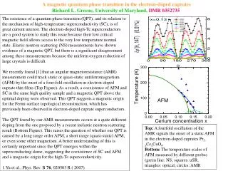
1. Motivation: Why Quantum Ferromagnets are Interesting Q: What happens to a FM phase transition when the Curie temperature is very low? A: Lots of unexpected and strange behavior. For instance: • The transition changes from second order to first order ZrZn2 (Uhlarz et al 2004) MnSi(Uemura et al 2007) Discontinuous magnetization Phase separation Chennai Lectures 2016
The phase diagram develops an interesting wing structure UGe2 (Kotegawa et al 2011) UCoAl (Aoki et al 2011) Chennai Lectures 2016
Quenched disorder suppresses these effects … • … leading to a continuous quantum phase transition … (Sang et al 2014) Ni3 Al1-x Ga2 (Yang et al 2011) Chennai Lectures 2016
… and for strong disorder to a quantum Griffiths region (Pikul 2012) (Westerkamp et al 2009) Chennai Lectures 2016
Non-Fermi-liquid transport behavior is observed in large regions of the phase diagram • Similar behavior is seen in many other quantum FMs (Takashima et al 2007) These lectures discuss some of these interesting effects. For a recent review, see M. Brando, DB, F.M. Grosche, TRK arXiv:1502.02898 Rev. Mod. Phys., in press Chennai Lectures 2016
2. Classical Phase Transitions a. Ferromagnets • The ferromagnetic transition in Fe, Ni, and Co is one of the best known examples of a thermal phase transition. • The material is a paramagnet at high temperatures, but spontaneously develops long-range ferromagnetic order if cooled below the Curie temperature Tc . • This transition in zero field is 2nd order; i.e. the order parameter (= magnetization) is a continuous function of temperature, but not analytic at T = Tc : • Mean-field theory (see below) qualitatively describes the data. • The transition at T < Tc as a function of a magnetic field is first order, i.e., the order parameter changes discontinuously. • Phase diagram: Ni (Weiss & Forrer 1926) Chennai Lectures 2016
50 years later: The true critical behavior is • M ~ (Tc – T) βwith β = 0.358 ± 0.003 • Order-parameter fluctuations invalidate mean-field theory near criticality in d=3, but NOT in a hypothetical system in d > 4 (Ginzburg criterion, “upper critical dimension”, see below). • Other critical quantities: • Exponent values depend only on the dimensionality and general properties (e.g., Ising vs Heisenberg), NOT on microscopic details (“universality classes”). Ni (Weiss & Forrer 1926) Cohen & Carver 1977 • Susceptibility 𝜒 ~ |T – Tc|-γwithγ≈ 1.4 • Correlation lengthξ ~ |T – Tc|-νwithν≈ 0.7 Chennai Lectures 2016
Theoretical explanation: Scaling, and the RG (Widom, Kadanoff, Wilson, Fisher, Wegner). • An important point: Scaling and the RG can be used to describe entire phases, not just critical points (“stable fixed points”, (e.g., Ma 1976) • Thermal fluctuations drive the critical singularities. • Observables obey homogeneity laws. E.g., with t = |T – Tc|/Tc and h the magnetic field, x x with b > 0 arbitrary • vs curves for various T will collapse onto ONE function with two branches if the axes are scaled appropriately! • This actually works (see next slide): Chennai Lectures 2016
CrBr3 (Ho & Litster 1969) Chennai Lectures 2016
“Action” (= Hamiltonian/T), partition function, free energy density for a classical FM: • Mean-field approximation, , • Landau free energy • 2nd order transition with mean-field exponents Chennai Lectures 2016
Focus on the susceptibility: • Homogeneous susceptibility: • Generalization to k > 0: x (Ornstein-Zernicke) x x correlation length • diverging length scale, LR correlations • Example of a “soft” or “massless” mode or excitation (here: a critical soft mode) • A time scale also diverges: (“critical slowing down”) • z is called “dynamical critical exponent” • Fluctuations 2nd order transition with exponents in the appropriate universality class (Ising, XY, or Heisenberg) • Fluctuations are important only below an upper critical dimension (d < 4 in this case); Ginzburg criterion Chennai Lectures 2016
Lecture 2 Chennai Lectures 2016
b. Liquid-gas transition • The liquid-gas transition maps onto an Ising ferromagnet, but we usually get to see only the 1st order transition. • Phase diagram: • The behavior near the critical point is in exact analogy to the ferromagnetic case. In particular, the correlation length diverges ( critical opalescence). • For T < Tc one observes phase separation. (Magnetic analogy: MnSi experiment) CO2 (Sengers & Levelt Sengers 1968) Chennai Lectures 2016
c. Superconductors (and liquid crystals) • Now consider a superconductor with order parameter : xx same as XY ferromagnet • But, couples to the E&M vector potential (photons): • A comes with a gradient A-correlation function diverges as : • Photons by themselves are soft (“generic” soft mode), but a nonzero gives them a mass! • “Integrate out” the photons: x x x with an “effective” action Chennai Lectures 2016
Treat in mean-field approximation The effective Landau free energy is • nonanalytic in : xx (Halperin, Lubensky, x Ma 1974) x • “Fluctuation-induced” 1st order transition! (NB: Fluctuations = generic soft modes!) • Nematic-Smectic-A transition in liquid crystals: Photons -> nematic Goldstone modes • Superconductors: effect is too weak to be observable; liquid Xtals: situation messy • Particle physics: “Coleman-Weinberg mechanism” Chennai Lectures 2016
3. Quantum Phase Transitions: General Concepts • Some ferromagnets have a low Tc that is often susceptible to hydrostatic pressure. • This raises the prospect of a quantum critical point at Tc = 0. • Quantum critical behavior is driven by quantum fluctuations must be different from classical critical behavior. • Crossovers ensure continuity. Q: How different is the description of QPTs in general from that of classical transitions? A: Very different, due to fundamental differences in statistical mechanics. Classical: QM: x x x x x statics and dynamics decouple! From DB, TRK, T. Vojta, Rev. Mod. Phys. 2005 Chennai Lectures 2016
Solution: Trotter formula • (Trotter 1959) • Coherent-state formalism (Casher, Lurie, Revzen 1969) • Divide the interval into infinitesimal slices, and integrate • End result: • is referred to as “imaginary time” (Wick rotation ) • Analytic continuation yields real-time (or frequency) dynamics • Statics and dynamics do indeed couple • If , then a quantum system in d spatial dimensions resembles a classical system in d + z dimensions! In general, (Hertz 1976) • Upper critical dimension of classical system implies • upper critical dimension of quantum system • Mean-field theory more robust in quantum case! Chennai Lectures 2016
4. The Quantum FM Transition in Metals, Part I: History • Stoner (1937): Mean-field theory for both classical and quantum case • Susceptibility: • RPA (“spin screening”) • with non-magnetic electrons • and the relevant interaction constant • Transition at (non-thermal control parameter) • Moriya et al (early 1970s): Self-consistent one-loop theory (aka self-consistent spin fluctuation theory) • Hertz (1976): Developed RG framework for QPTs in general, used metallic FMs as a prime example. • Millis (1993): Used Hertz’s RG framework to determine temperature scaling. • Plausibility arguments for Hertz’s action (with a lot of hindsight): • Landau free energy (again): • t is the inverse physical (dressed) susceptibility 1/ x Chennai Lectures 2016
RPA again: • Generalize everything to nonzero wavevectors (Fourier trafo of ) • and frequencies (Fourier trafo of ) x • holds for noninteracting electrons • x (Lindhard fct) AND for interacting ones • action • describes the dynamics of clean electrons (“Landau damping”) • Represents coupling of conduction electrons dynamics to the magnetization • At • for classical magnets implies • for quantum magnets • Conclusion (as of 1976): Mean-field theory yields exact critical behavior for all d > 1 ( QPTs not very interesting as far as critical behavior goes) Chennai Lectures 2016
As mentioned before, this is not what is observed experimentally. • In most clean systems, the transition becomes first order if Tc is suppressed far enough • Examples: • There are many others: ZrZn2 Uhlarz et al 2004 • ZrZn2(Uhlarz et al 2004) • MnSi (Pfleiderer et al 1997, Uemura et al 2007) • UGe2 (Aoki et al 2011) Uemura et al 2007 Chennai Lectures 2016
There are many more examples (Brando et al, Rev Mod Phys in press) Chennai Lectures 2016
5. The Quantum FM Transition, Part II: General Guidelines • Observations: • A tricritical point separates the 2nd order transitions from the 1st order ones. • In a magnetic field, tricritical wings appear: • A quantum critical point is eventually realized, but only at a nonzero magnetic field! • This behavior is seen in systems that are very different with respect to electronic structure, type of magnet (Ising, XY, Heisenberg), etc. • The explanation must be universal, i.e., a lie in stat. mech., not in solid-state effects. • Look for an explanation that involves x low-lying excitations (aka soft modes) • These materials are all metals Conduction electrons likely important • Study Fermi liquids first. • Q: Don’t we know everything about Fermi liquids, and wasn’t that built into Hertz’s x action? • A: NO! (Kotegawa et al 2011) Chennai Lectures 2016
Spoiler: The answer in a nutshell: A novel type of fluctuation-induced 1stx order transition • The leading wavenumber dependence of the inverse susceptibility that enters the action is x for 1 < d < 3 and x for d = 3 • This is a consequence of soft modes in a Fermi liquid, see below • Scaling suggests h ~ k, so this nonanalyticity is also present for at k = 0 as a function of h. • The magnetization is seen by the conduction electrons as an effective field. • In a generalized Landau theory, translates into • This leads to a generalized Landau free energy x x with x which leads to a 1st-order transition. • Conclusion: In clean metals, generic soft modes couple to the ferromagnetic order parameter and make the quantum FM transition generically 1st order. (DB, TRK, T. Vojta 1999) Chennai Lectures 2016
Lecture 3 Chennai Lectures 2016
6. The Fermi Liquid as an Ordered Phase a. A useful example: Classical ϕ4 – theory(again) • O(3) ϕ4 – theoryin d spatial dimensions with a field in 1-direction: • Saddle-point solution for the ordered phase: • with x • Fluctuations: Chennai Lectures 2016
Properties of the ordered phase: Reduction due to fluctuations • Magnetization • Transverse susceptibility • Longitudinal and transverse modes couple • x nonanalyticities • First derived in perturbation theory (Vaks, Larkin, Pikin 1967, x Brézin & Wallace 1973) • Exact result, governed by Ward identity • Transverse fluctuations are soft (Goldstone modes of the spontaneously broken SO(3) ) • Longitudinal fluctuations are massive Potential for SO(2) ≅ U(1) (planar magnet) Long-ranged correlations! Chennai Lectures 2016
Derivation via RG methods: • Expand in powers of fluctuations and gradients, assign scale dimensions, and look for a stable fixed point. • The above behavior is exact for all d > 2 and can be described by a • Fixed-point action x dimensionless • plus least irrelevant operators, e.g. • This suffices for deriving all scaling behaviors, e.g. • Nonanalyticities are leading corrections to scaling at the stable fixed point • d = 2 is lower critical dimension (Mermin-Wagner ✔ ) Chennai Lectures 2016
Note: Similar arguments can be used to exactly characterize nonanalyticities in various other systems, both classical and quantum. For instance, • The shear viscosity in classical fluids has a nonanalytic frequency dependence since it couples to the diffusive transverse-velocity fluctuations. • This is an example of classical long-time tails, i.e., non-exponential decay of correlation functions. • The conductivity at T = 0 in a disordered metal is a nonanalytic function of the frequency • This is an example of what are called weak-localization and Altshuler-Aronov effects in disordered metals. • We will now apply analogous arguments to a clean Fermi liquid. Chennai Lectures 2016
b. Goldstone modes in a Fermi liquid (i) The stable Fermi-liquid fixed point • A long story (Wegner 1970s, TRK & DB 1997, 2012) made very short: • In a Fermi system at T = 0, there are two-particle excitations that are • The Fermi liquid is an ordered phase characterized by • the soft modes (analogous to π ) that • These soft modes are the clean analogs of what are called “(spin)-diffusons” in disordered systems, where they lead to weak-localization and Altshuler-Aronov effects. (They are NOT density fluctuations.) • are controlled by a Ward identity • are Goldstone modes of a spontaneously broken symmetry • have a linear dispersion relation • acquire a mass at T > 0 and h > 0 Chennai Lectures 2016
an order parameter given by the DOS at the Fermi surface (more precisely: By the spectrum of the Green’s function): • an order-parameter susceptibility (analogous to ) • a stable RG fixed point with fixed-point action • all other terms are x RG irrelevant! a • Scale dimensions • Least irrelevant operators • with scale dimension • This allows for the derivation of homogeneity laws that yield the exact leading nonanalyticities in a Fermi liquid! Chennai Lectures 2016
(ii) Universal properties of the Fermi liquid • DOS: • Spin susceptibility: Jiang et al 2006 • analogous to • agrees with perturbative results (Khveshchenko & Reizer 1998) • first derived in perturbation theory (DB, TRK, T Vojta 1997; Betouras et al 2005) • NB the sign of the effect! • Soft modes long-ranged correlations nonanalytic behavior Chennai Lectures 2016
7. The Quantum Ferromagnetic Transition, Part III a. Generalized Landau theory • Ordinary Landau theory: • with t = 1/ the inverse susceptibility • Now recall the argument given earlier: • The FL Goldstone modes lead to a generalized Landau theory: • acts as an effective field • in a metal, the FL Goldstone modes couple to via a Zeeman term • via the nonanalytic h – dependence of ! x The quantum ferromagnetic transition in clean metals in zero field is generically 1st order ! Chennai Lectures 2016
Other consequences: • T > 0 gives Goldstone modes a mass xtricritical point • Magnetic field h > 0tricritical wings • Generic phase diagram: • Predicted to hold for all clean metallic • Third Law General constraints on the shape of the phase diagram (see my Colloquium talk) • Pre-asymptotic region: Crossover to Hertz-Millis-Moriya behavior. Example: MnSi • Comparison with experiments: Excellent qualitative agreement. The transition in clean materials is generically 1st order. In some systems (e.g., NixPd1-x) the transition needs to be followed to lower T. • Ferromagnets (isotropic or anisotropic, itinerant or not, and even Kondo lattices) • Ferrimagnets (only requirement is a homogeneous magnetization component) • Magnetic nematics (DB, TRK, J Rollbühler 2005) (Pfleiderer et al 1997) Chennai Lectures 2016
b. Order-parameter fluctuations • Technical derivation: Coupled field theory for fermions and OP fluctuations. • Q: How good or bad is the mean-field approximation? • A: Nobody really knows, but: • Treat conduction electrons in a tree approximation Hertz’s action • 1-loop order nonanalyticities appear • Higher order: Only prefactors change • OP fluctuations are above their upper critical dimension • In liquid crystals, they are below the upper critical dimension • This makes it plausible that the 1st order transition in quantum ferromagnets is much more robust than in liquid crystals. Other suggestions for avoiding a quantum critical point : • Textured phases (spiral, etc), with the length scale set by the maximum in (Chubukov et al, Green et al) Chennai Lectures 2016
c. Effects of quenched disorder Quenched disorder changes things drastically: • The generic soft modes are now diffusive • The susceptibility now is x x(Altshuler et al early 1980s)NB the sign! x and by the same arguments as before we have, in d = 3, • (TRK & DB 1996) • This predicts a 2nd order transition with non-mean-field exponents. • For instance, , and , consistent with many observed phase diagrams (see below for other interpretations) • Order-parameter fluctuations lead to log-normal modifications of the power laws (DB et al 2001) • Increasing the disorder from the clean limit decreases the tricritical temperature continuously (Pikul et al 2012) Chennai Lectures 2016
Prediction for evolution of phase diagram: • Quantum Griffiths effects (McCoy & Wu 1968, D.S. Fisher 1995) • Based on the idea of the classical Griffiths region below the clean Tc. Diverging susceptibilities without long-range order. • Quantum version may coexist with, and be superimposed on, quantum critical behavior (Millis et al, Randeria et al, T. Vojta, …) • Experiments have been interpreted using these concepts, e.g. Complications for strong disorder: (Sang et al 2014) (Westerkamp et al 2009) (Pikul 2012) Chennai Lectures 2016
Lecture 4 Chennai Lectures 2016
8. Exponents and Exponent Relations at Quantum Critical x Points Now consider a continuous QPT, e.g. the FM one in Ni3 Al1-x Ga2: A classical critical point is characterized by power-law behavior of observables, and corresponding critical exponents: Order parameter: Order-parameter susceptibility: Correlation length: Specific heat: Chennai Lectures 2016
A quantum critical point we can approach at T = 0 by varying the non-thermal control parameter t, or at t = 0 by letting T -> 0. • We need more critical exponents! • Order parameter: • Order-parameter susceptibility: • Correlation length: • The specific heat vanishes at T = 0 => Consider the • Specific-heat coefficient: Chennai Lectures 2016
The T- exponents will in general be different from the t- exponents! What is the relation? Various points towards an answer: • In quantum statistical mechanics, inverse temperature is related to (imaginary) time. => T- scaling is governed by a dynamical exponent z that describes how the relaxation time diverges as a function of the relaxation length: • Power laws result from generalized homogeneity laws for observables : • with b an arbitrary length rescaling factor and a scaling function x (and r = t, sorry!). • Put b = r-ν => • At r = 0 we have • with • Conclusion: If describes the static scaling behavior, then • describes the temperature scaling behavior • Caveat: This is true only under special circumstances. More generally, the T-scaling of may be described by A z, rather than by THE z, due to multiple time scales and/or dangerous irrelevant variables. Chennai Lectures 2016
That’s a lot of exponents. How many are independent? First consider a classical transition. Look at the homogeneity law for the order parameter: => ✓ ✓ Now, the susceptibility is a thermodynamic derivative of : This yields => => “Widom’s equality” Similar arguments lead to, e.g., “Essam-Fisher equality” “Fisher equality” Chennai Lectures 2016
Some exponent relations depend explicitly on the dimensionality, e.g. “hyperscaling” They are not valid if the dimensionality is larger than the “upper critical dimension”. For many classical transitions, that’s d = 4. Classically, only two exponents are independent. These exponent relations all depend on various forms of scaling being valid. While that’s usually the case at critical points, there is no guarantee. Weaker statements that depend only on thermodynamic stability take the form of rigorous inequalities. For instance, “Rushbrooke inequality” In disordered systems, a rigorous lower bound on the correlation length exponent is known: Chayes, Chayes, Spencer, Fisher (1986) (See also the “Harris criterion”). Chennai Lectures 2016
At quantum critical points, some of the classical relations still hold, e.g., Widom Fisher Analogous relations hold for the T- exponents: Others change. For instance, a generalization of Essam-Fisher becomes where and are the dynamical exponents that govern the T – dependence of the order parameter and the specific heat, respectively. These two are in general NOT the same! The rigorous Rushbrooke inequality holds for the T – exponents: but gets modified for the t – exponents: Chennai Lectures 2016
Hyperscaling relations, e.g., again hold only below some upper critical dimensionality, which tends to be lower for quantum phase transitions than for classical ones. Overall, at a quantum critical point there are at least two independent static critical exponents, plus the dynamical ones. Depending on what form of scaling holds (which depends on the critical point and the dimensionality) there may be as many as five independent static exponents. For details, see Chennai Lectures 2016
9. “How Close is Close to the Critical Point?”, or x How Hard is it to Measure Quantum Critical Exponents? Q: How close to the critical point does one have to go in order to observe asymptotic critical behavior? A: It depends on the critical point and the observable, but in general very close. At many classical critical points one needs to be closer than 0.1%, and then one needs two or three decades to convincingly see the power laws! Plus, the extracted exponent values can depend strongly on the value of Tc! Chennai Lectures 2016
Farther away from criticality one often observes effective power laws with exponents that are controlled by unstable RG fixed points. • There is no reason to believe that requirements at quantum critical points are less stringent. Various issues: • Many quantum critical points are controlled by chemical composition. This is hard to control, and the critical concentration is typically not known very precisely. • Additional physics can mask quantum criticality, e.g., quantum Griffiths effects in many disordered quantum ferromagnets. Chennai Lectures 2016