Download
1 / 25
250 likes | 312 Views
This chapter aims to enhance students' understanding of the cosmic background across electromagnetic spectrum frequencies. It covers effects of IGM, absorption, and interaction with photons, discussing known objects and undetected populations. Topics include radiation, objects distribution, conservation laws, Olber’s Paradox, and X-ray background exploration, referring to related research and observations. Revisitations on reheating processes post-recombination and Compton scattering effects on microwave background are also covered.

E N D
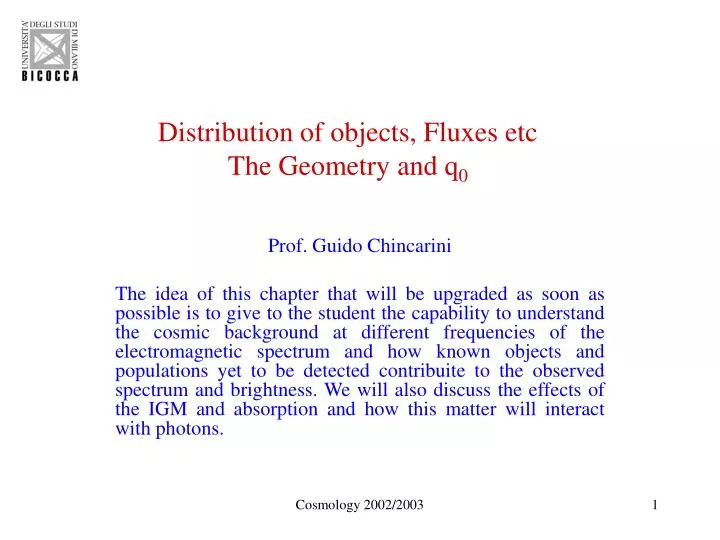
Distribution of objects, Fluxes etcThe Geometry and q0 Prof. Guido Chincarini The idea of this chapter that will be upgraded as soon as possible is to give to the student the capability to understand the cosmic background at different frequencies of the electromagnetic spectrum and how known objects and populations yet to be detected contribuite to the observed spectrum and brightness. We will also discuss the effects of the IGM and absorption and how this matter will interact with photons. Cosmology 2002/2003
Counts - = 0.0 m=0.1 m=0.2 m =0.4 Cosmology 2002/2003
And adding m=0.3 m=0.7 Cosmology 2002/2003
Radiation by background objects Definitions: j => emissivity in erg cm-3 s-1 Hz-1 z1 z2 => redshift interval over which the sources are dsitributed. U => density of energy in erg cm-3 Hz-1 H(z) => Hubble constant at the epoch z I => Intensity in units ergs cm-3 s-1 Hz-1 sr-1 dL/d = L0 - spectral distribution between min and max for a sample of sources Also we should recall that the Volume goes as (1+z)3. Better we will show that I/3 is an invariant. Cosmology 2002/2003
Conservation Consider a stream of particle propagating freely in the space time. A comoving observer at the time t finds dN particle in the comoving volume dV. These have momentum in the range p p+dp3. Using the phase distribution function f(x,p,t) we can write dN=f dV dp3. At a later time, t+dt, the proper volume is increased by a factor [a(t+dt)/a(t)]3 and the volume in the momentum space {we have shown a few lectures ago velocity (or momentum) a-1 See the Chapter the Hubble expansion and the cosmic redshift} goes as [a(t)/a(t+dt)]3 so that the phase volume occupied by the particles does not change during the free propagation. Since the number of particles is also conserved it follows that the phase space distribution function is conserved along the streamline. We can use a similar reasoning for photons where we also showed that the frequency changes (redshift) as a function of the expansion. Cosmology 2002/2003
We can reason using photons • For photons we can demonstrate an important invariant in a similar way. In this case we can write the momentum space volume as dp3 p2dpd 2 d d and dx3 cdt dA {dA is the area normal to the direction of propagation}. Using the subscript e for the emission and the subscript r to indicate the photons received by the surface we can write for the conserved number of photons per unit phase space volume: Cosmology 2002/2003
From this it follows: Cosmology 2002/2003
Olber’s Paradox Density of Objects The flux I receive from each star or galaxy But the Night Sky is Dark Cosmology 2002/2003
X ray Background - Preliminaries • The discovery goes back to Giacconi et al. (1962) Cosmology 2002/2003
The X ray Backgroundsee also Peacock Page 358 and Steeve Holt – See Math X_Bck Here kT = 40 keV. If we subtract a source density of a density of about 400 sources deg-2 (2.5 10-18 W m-2) that accounts for 60% of the Background we have the relation below with 0 < < 0.2 [TBChecked] and kT about 23 – 30- keV. Cosmology 2002/2003
The Plots – (See Math X_Bck) Fit of the Background Cosmology 2002/2003
Home work • The class or the student developes all this part according to the latest observations related to the Chandra deep field etc. • References: • Hasinger Cosmology 2002/2003
How could we explain an X ray background anyhow The Universe after recombination must go through a reheating process. The main reason for this is that the Universe is completely transparent to radiation and HI is not detected. On the other hand the structure formation process can not have been 100% efficient so that HI should have been left around. Recombination occurs at z ~ 1000 and the gas Temperature, for a gas we can use = 5/3 and for Radiation = 4/3 , according to the adiabatic expansion T R-3 (-1) and therefore T a-2. Guilbert and Fabian (1986, MNRAS 220, 439) estimate To = 3.6 keV and gash2 ~ 0.24 assuming reheating at redshift z=6 [This also should be revisited for reheating may be at higher redshift]. Note that if the gas is clumped the density is higher in the emitting region since Bremsstrahlung goes as n2. Cosmology 2002/2003
The y parameter If we have a gas at very high energy the Compton inverse effect will be very strong. The electron hits a photon and convert a low energy photon to a high energy photon by a factor of the order 2 in the case of relativistic electrons. This type of scattering would cause a distortion in the Microwave Spectrum (see also the Sunayev Zeldovich effect) by depopulating the Rayleigh Jeans regime in favour of photons in the Wien tail. On the other hand the observations of the Microwave Background is thermal to an extremely high degree of accuracy (COBE and WMAP) so that we can rule out models with too much hot gas. According to Fixsen et al. 1996 Ap J 473, 576 COBE sets a limit of y<1.5 10-5. It is very important to estimate if there is any background at all. If present we may have too look into the emission by a population of low luminosity active galaxies. Something it is worth searching for. Cosmology 2002/2003
Numbers now Cosmology 2002/2003
Conclusions • Using the limit given by COBE we derive zmax <0.1 in contraddiction with the fact that reheating is at high redshift, larger than z. This to account fot the X ray Background. • We might have a rather clumped gas. The X ray emission scale with the parameter f = <ne2>/<ne>2 and we should have f >104. In this case however we must make a model for the evolution of the temperature in the clumps. • If the background is made out of discrete sources then need to have a density of about 5000 sources per squaredegree [TBC]. We do not have that many clusters of galaxies and that is why we are considering active low luminosity galaxies. • It is very clear that the next X ray observations must give a detailed number counts of sources. To do that we need a fairly good resolution. Cosmology 2002/2003
HI – 21 cm The emission of the neutral Hydrogen could be written as j()=(3/4) A nH h (-H). A=2.85 10-15 s-1 nH = n0 (1+z)3 [1-x(z)] ; x(z) fraction of ionized gas at z. n0 present number density of hydrogen atoms + ions. In the expanding Universe we will: • Observe the flus at all frequencies with 0 < H and no Flux at 0 > H • The discontinuity is given by [possibly derive this]: Cosmology 2002/2003
Expansion and AbsorptionQuestion: What is the Optical depth due to matter in theredshift range 0 to z Absorption will take place anywhere between 0 and zsource and the flux will be diminished at all frequencies in the band H/(1+z) and H. The discontinuity will be given by: Cosmology 2002/2003
The q0 Dust Universe Cosmology 2002/2003
0 For small a(t) the term in can be disregarded, it will dominate for large values of a. And this becomes a puzzle, we are in the right epoch to be capable of measuring because it is now the dominating term. If <0 a can not become extremely large since da/dt must be real. For this value of acrit = Max size. Cosmology 2002/2003
> 0 • K=0 or K=-1 • For a(t) large the model enter a phase of exponential expansion – The equation becomes • K=+1 We need a fine tuning among the different terms. • We could fine tune to have da/dt=0 and d2a/dt2 =0 (static model) • For larger the repulsive force dominates and the Universe will expand forever • For smaller we find a range with a<0. These values are therefore forbidden. • Etc The student practice. Cosmology 2002/2003
< 0 = 0 k=-1 k= 0 k=+1 t Cosmology 2002/2003
> 0 k=-1 k= 0 c >> 0 > c k=+1 = c t Cosmology 2002/2003