Download
1 / 63
650 likes | 834 Views
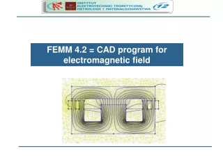
FEMM is a suite of programs for solving low-frequency electromagnetic problems in planar and axisymmetric domains. It includes interactive shell, CAD-like interface, and field visualization capabilities. The finite element method is used to approximate solutions for various types of problems.

E N D
Introduction to FEM • FEMM is a suite of programs for solving lowfrequency electromagnetic problems on two-dimensional planar and axisymmetric domains. The program currently addresses • linear/nonlinear magnetostatic problems, • linear/nonlinear time harmonic magnetic problems • linear electrostatic problems, • steady-state heat flow problems. 02/01/2020 17:22
FEMM is divided into three parts: • Interactive shell (pre-processor and a post-processor for the various types of problems solved by FEMM 4.2 . • CADlike interface for laying out the geometry of the problem to be solved and for defining material properties and boundary conditions. • Field solutions can be displayed in the form of contour and density plots. • The program allows the user to inspect the field at arbitrary points, as well as evaluate a number of different integrals and plot various quantities of interest along user-defined contours. • Triangle.exe breaks down the solution region into a large number of triangles, a vital part of the finite element process. • Solvers (fkern.exe for magnetics; belasolv for electrostatics); Each solver takes a set of data files that describe problem and solves the relevant partial differential equations to obtain values for the desiredfield throughout the solution domain. 02/01/2020 17:22
The idea of finite elements • to break the problem down into a large number of regions, each with a simple geometry (e.g. triangles). • over these simple regions, the “true” solution for desired potential is approximated by a very simple function. • the advantage of breaking the domain down into a number of small elements: • the problem becomes transformed from a small but difficult to solve into a big but relatively easyto solve.
Example of the planar electrostatic model 02/01/2020 17:22
Presentación FEM analysis, example of discretization 02/01/2020 17:22
Presentación Some posibilities 02/01/2020 17:22
FEM • The finite element method (FEM) (finite element analysis (FEA)) is a numerical techniques for finding approximate solutions of partial differential equations (PDE) as well as of integral equations. • The solution approach is based either on eliminating the differential equation completely (steady state problems) or rendering the PDE into an approximating system of ordinary differential equations, which are then numerically integrated using standard techniques such as Euler's method, Runge-Kutta,….
Tipos de problema Electrostatic problems • The behavior of electric field intensity E, and electric flux density (alternatively electric displacement or induction) D. • The program solves for voltage V over a user-defined domain with user-defined sources and boundary conditions. 02/01/2020 17:22
Diseño New problem initial data • Problem types: • planar (cartesian coordinates); • axisymmetric (cylindrical coordinates) • Length units: mm, cm and m.. • “Depth” = third dimention of the investigated object. Minimum angle of the triangle element,(value from 1 to 33,8 deg) 02/01/2020 17:22
Snap to grid Grid on/off Grid properties button New problem definition, GRID 02/01/2020 17:22
Preprocessor Drawing ModesPreprocessor Drawing Modes Adding “Block Label” markers into each section of the model to define material properties and mesh sizing for each section.. Drawing the endpoints of the lines and arc segments that make up a drawing. Connecting the endpoints with either line segments or arc segments 02/01/2020 17:22
shortcuts and mouse buttons (for point properties) Double click: Display coordinates of the nearest point Select the nearest point Create a new point at the current mouse pointer location Delete selected points Unselect all points Display dialog for the numerical entry of coordinates for a new point Edit the properties of selected point(s) SPACE KEY 02/01/2020 17:22
Some operations Parameters for moving, copying, rotating Example of 60º element rotation Copy Rescale Move Symmetry Area selection Delete 02/01/2020 17:22
Electrostatic problems Materials choosed for actual analysis 02/01/2020 17:22 Transparencia nº 15
Properties of the materials • New material creation. 02/01/2020 17:22
Line properties for electrostatic problems 02/01/2020 17:22
allow the user to apply constraints on the total amount of charge carried on a conductor. Alternatively, conductors with a fixed voltage can be defined, and the program will compute the total charge carried on the conductor during the solution process. 02/01/2020 17:22
boxes for defining the voltage at a given point, or prescribing a point charge density at a given point. 02/01/2020 17:22
Electrostatica Electrostatic analysis Manual choice of mesh size Output (graphical postprocessor) Start calculations Building triangles (meshes) 02/01/2020 17:22
Posprocesador Possibilities of the electrostatic postprocessor Zoom in/out Result visualisation (density plots, equipotential lines, vectors) Shifting the screen Selection of numerical method and visualisation Selection of points, lines or blocks for numerical analysis and graphical presentation Grid parameters Open problem or start a new problem 02/01/2020 17:22
Point properties (electrostatic postprocessor) Output results Output selection: point 02/01/2020 17:22
Graphical postprocessor Plot the function plot Choose the type of field value 02/01/2020 17:22
Line integral Definition of the line Options Integral results Start of the integration 02/01/2020 17:22
Posprocesador Block element options result Block Integrals To select the regions over which a block integral is to be performed, left-click with the mouse in the desired region. The selected region will appear highlighted in green. Start button 02/01/2020 17:22
Electrostatics Postprocessor: Equipotential lines options Visualisation dialog box 02/01/2020 17:22
Electrostatics Postprocessor:Density plots Electric field area Legend Menu 02/01/2020 17:22
Posprocesador Electrostatics Postprocessor:Vector plots Vectors START Dialog box 02/01/2020 17:22
Step by step EXAMPLE 1 • Capacitor with a Square Cross-Section
The outer square has a 4 cm size, the inner square2 cm size. • The geometry extends for 100 cm in the “into-the-page” direction. • The dielectricbetween the plates air. • TASK: build the FEMM problem (model), analyze it, and determine the capacitance.
Procedure • Physical problem description. • Model design. • Boundaries definition. • Materials description. • Boundary conditions application. • Mess generation. • Finite Element Method application. • Results extraction and analysis.
The finished model Remark: Because of the symmetry, only one quarter of the device need to be modeled.
Create model • Start FEMM "File|New" from the main menu. • Select "Electrostatics Problem" in the"Create a new problem" dialog that appears. • After you hit "OK", a blank electrostatics problemwill appear.
Press <TAB> BUTTON Enter x=0, y=2 Select „nodes” Entered POINT (0,2)
To select the endpoint of a line, click near desired endpoint with the left mouse button! Select „lines” and try to connect all points
Add materials to the model • Select „Properties|Materials” • Click Add Materials” • Change the name of the property to „AIR” • Confirm by clicking „OK.”
Define materials for each region • Click „Block Labels” • It can be done via <TAB> dialog or by click on the left button • Make block label red (right click) • Press space to „oopen” the selected block label • Set to AIR • Uncheck „Let Triangle….” • Choose Mesh Size „0.025”
SPACE BUTTON Right click
Define conductor voltages • Select „Properties| Conductors” • Click „Add Property” • Replace „New Conductor” with „ZERO” • Select „Prescribed Voltage”, enter „0”, confirm • Repeat the above procedure to the new boundary condition „ONE” • Attribute conductor voltages to the segments • When segment turns to red press SPACE BAR and change the selction from „none” to „ZERO” or „ONE”
PRESS SPACE BAR
Set PROBLEM Characteristics • Select „Problem” • Choose „planar” • Set the length units to „Centimeters” • Depth = 100 • Default solver precicion (10-8)
GENERATE MESH and RUN! • Save the file • Click button with yellow mesh • If the mesh seems to be to fine or too coarse select mesh size again • „TURN the CRANK”