Download
1 / 36
360 likes | 380 Views
Explore the mapping and inverse mapping of signals using complex cepstrum, determination of complex cepstrum for minimum-phase signals, and deconvolution techniques for signal separation. Learn about homomorphic systems, Fourier transforms, and frequency-invariant linear filtering.

E N D
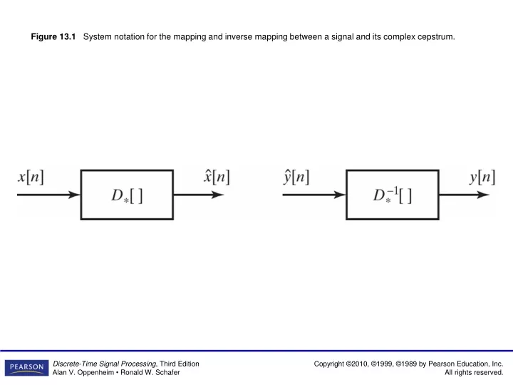
Figure 13.1 System notation for the mapping and inverse mapping between a signal and its complex cepstrum.
Figure 13.2 Determination of the complex cepstrum for minimum-phase signals.
Figure 13.3 Cascade of three systems implementing the computation of the complex cepstrum operation D∗[ ].
Figure 13.4 Approximate realization using the DFT of (a) D∗[・] and (b) D−∗1 [・].
Figure 13.5 (a) Samples of arg[X(ejω)]. (b) Principal value of part (a). (c) Correction sequence for obtaining arg from ARG.
Figure 13.6 Canonic form for homomorphic systems where inputs and corresponding outputs are combined by convolution.
Figure 13.7 Deconvolution of a sequence into minimum-phase and allpass components using the cepstrum.
Figure 13.8 The use of homomorphic deconvolution to separate a sequence into minimum-phase and maximum-phase components.
Figure 13.9 Pole-zero plot of the z -transform X(z) = V(z)P(z) for the example signal of Figure 13.10.
Figure 13.10 The sequences: (a) v[n], (b) p[n], and (c) x[n] corresponding to the pole–zero plot of Figure 13.9.
Figure 13.11 The sequences: (a) v[n], (b) p[n], and (c) x[n]. ˆ ˆ ˆ
Figure 13.12 The sequences: (a) cv[n], (b) cp[n], and (c) cx[n].
Figure 13.13 Fourier transforms of x[n] in Figure 13.10. (a) Log magnitude. (b) Principal value of the phase. (c) Continuous “unwrapped” phase after removing a linear-phase component from part (b). The DFT samples are connected by straight lines.
Figure 13.14 (a) Complex cepstrum xp[n] of sequence in Figure 13.10(c). (b) Cepstrum cx[n] of sequence inFigure 13.10(c). ˆ
Figure 13.15 (a) System for homomorphic deconvolution. (b) Time-domain representation of frequency-invariant filtering.
Figure 13.16 Time response of frequency-invariant linear systems for homomorphic deconvolution. (a) Lowpass system. (b) Highpass system. (Solid line indicates envelope of the sequence [n] as it would be applied in a DFT implementation. The dashed line indicates the periodic extension.)
Figure 13.17 Lowpass frequency-invariant linear filtering in the system of Figure 13.15. (a) Real parts of the Fourier transforms of the input (solid line) and output (dashed line) of the lowpass system with N1 = 14 and N2 = 14 in Figure 13.16(a). (b) Imaginary parts of the input (solid line) and output (dashed line). (c) Output sequence y [n] for the input ofFigure 13.10(c).
Figure 13.18 Illustration of highpass frequency-invariant linear filtering in the system of Figure 13.15. (a) Real part ofthe Fourier transform of the output of the highpass frequency-invariant system with N1 = 14 and N2 = 512 in Figure 13.16(b). (b) Imaginary part for conditions of part (a). (c) Output sequence y [n] for the input of Figure 13.10.
Figure 13.19 (a) Complex cepstrum of x[n] = xminn∗xap[n]. (b) Complex cepstrum of xmin[n]. (c) Complex cepstrum of xap[n].
Figure 13.20 (a) Minimum-phase output. (b) Allpass output obtained as depicted in Figure 13.7.
Figure 13.21 (a) Minimum-phase output. (b) Maximum-phase output obtained as depicted in Figure 13.8.
Figure 13.23 Homomorphic deconvolution of speech. (a) Segment of speech weighted by a Hamming window. (b) High quefrency component of the signal in (a). (c) Low quefrency component of the signal in (a).
Figure 13.24 Complex logarithm of the signal of Figure 13.23(a): (a) Log magnitude. (b) Unwrapped phase.
Figure 13.25 Complex cepstrum of the signal in Figure 13.23(a) (inverse DTFT of the complex logarithm in Figure 13.24).
Figure 13.26 (a) System for cepstrum analysis of speech signals. (b) Analysis for voice speech. (c) Analysis for unvoiced speech.
Figure 13.27 (a) Cepstra and (b) log spectra for sequential segments of voiced speech.