Download

1 / 48
480 likes | 602 Views
4: Probability. Part A: Concepts & binomial distributions Part B: Normal distributions. Definitions. Random variable a numerical quantity that takes on different values depending on chance Population the set of all possible values for a random variable

E N D
4: Probability Part A: Concepts & binomial distributions Part B: Normal distributions Unit 4: Intro to probability
Definitions • Random variable a numerical quantity that takes on different values depending on chance • Population the set of all possible values for a random variable • Event an outcome or set of outcomes for a random variable • Probability the proportion of times an event occurs in the population; (long-run) expected proportion Unit 4: Intro to probability
Probability (definition #1) The probability of an event is its relative frequency (proportion) in the population. Example: Let A selecting a female at random from an HIV+ population There are 600 people in the population. There are 159 females. Therefore, Pr(A) = 159 ÷ 600 = 0.265 Unit 4: Intro to probability
Probability (definition #2) The probability of an event is its expected proportion when the process in repeated again and again under the same conditions • Select 100 individuals at random • 24 are female • Pr(A) 24 ÷ 100 = 0.24 • This is only an estimate (unless n is very very big) Unit 4: Intro to probability
Probability (definition #3) The probability of an event is a quantifiable level of belief between 0 and 1 Example: Prior experience suggests a quarter of population is female. Therefore, Pr(A) ≈ 0.25 Unit 4: Intro to probability
Some rules of probability Unit 4: Intro to probability
Types of random variables • Discrete have a finite set of possible outcomes, • e.g. number of females in a sample of size n (0, 1, 2, …, n) • We cover binomial random variables • Continuous have a continuum of possible outcomes • e.g., average body weight (lbs) in a sample (160, 160.5, 160.75, 160.825, …) • We cover Normal random variables There are other random variable families, but only binomial and Normal RVs are covered for now. Unit 4: Intro to probability
Binomial distributions • Most popular type of discrete RV • Based on Bernoulli trial random event characterized by “success” or “failure” • Examples • Coin flip (heads or tails) • Survival (yes or no) Unit 4: Intro to probability
Binomial random variables • Binomial random variable random number of successes in n independent Bernoulli trials • A family of distributions identified by two parameters • n number of trials • p probability of success for each trial • Notation: X~b(n,p) • X random variable • ~ “distributed as” • b(n, p) binomial RV with parameters n and p Unit 4: Intro to probability
“Four patients” example • A treatment is successful 75% of time • We treat 4 patients • X random number of successes, which varies 0, 1, 2, 3, or 4 depending on binomial distribution X~b(4, 0.75) Unit 4: Intro to probability
The probability of i successes is … Binomial formula Where nCi= the binomial coefficient (next slide) p = probability of success for each trial q = probability of failure =1 – p Unit 4: Intro to probability
Binomial coefficient (“choose function”) where ! the factorial function: x! = x (x – 1) (x – 2) … 1 Example: 4! = 4 3 2 1 = 24 By definition 1! = 1 and 0! = 1 nCi the number of ways to choose i items out of n Example: “4 choose 2”: Unit 4: Intro to probability
“Four patients” example • n = 4 and p = 0.75 (so q = 1 - 0.75 = 0.25) • Question: What is probability of 0 successes? i = 0 • Pr(X = 0) =nCi pi qn–i = 4C0 · 0.750 · 0.254–0= 1 · 1 · 0.0039 = 0.0039 Unit 4: Intro to probability
X~b(4,0.75), continued Pr(X = 1) = 4C1· 0.751 · 0.254–1 = 4 · 0.75 · 0.0156 = 0.0469 Pr(X = 2) = 4C2· 0.752 · 0.254–2 = 6 · 0.5625 · 0.0625 = 0.2106 (Do not demonstrate all calculations. Students should prove to themselves they derive and interpret these values.) Unit 4: Intro to probability
X~b(4, 0.75) continued Pr(X = 3) = 4C3· 0.753 · 0.254–3 = 4 · 0.4219 · 0.25 = 0.4219 Pr(X = 4) = 4C4· 0.754 · 0.254–4 = 1 · 0.3164 · 1 = 0.3164 Unit 4: Intro to probability
The distribution X~b(4, 0.75) Probability table for X~b(4,.75) Probability curve for X~b(4,.75) Unit 4: Intro to probability
Get it? Pr(X = 2) = .2109 Area under the curve (AUC) concept The area under a probability curve (AUC) = probability! Unit 4: Intro to probability
Cumulative probability (left tail) • Cumulative probability = Pr(X i) = probability less than or equal to i • Illustrative example: X~b(4, .75) • Pr(X 0) = Pr(X = 0) = .0039 • Pr(X 1) = Pr(X 0) + Pr(X = 1) = .0039 + .0469 = 0.0508 • Pr(X 2) = Pr(X 1) + Pr(X = 2) = .0508 + .2109 = 0.2617 • Pr(X 3) = Pr(X 2) + Pr(X = 3) = .2617 + .4219 = 0.6836 • Pr(X 4) = Pr(X 3) + Pr(X = 4) = .6836 + .3164 = 1.0000 Unit 4: Intro to probability
X~b(4, 0.75) Unit 4: Intro to probability
Bring it on! Cumulative probability left tail = cumulative probability Area under shaded bars in left tail sums to 0.2617, i.e., Pr(X 2) = 0.2617 Area under “curve” = probability Unit 4: Intro to probability
Reasoning Use probability model to reasoning about chance. I hypothesize p = 0.75, but observe only 2 successes. Should I doubt my hypothesis? ANS: No. When p = 0.75, you’ll see 2 or fewer successes 25% of the time (not that unusual). Unit 4: Intro to probability
StaTable probability calculator • Link on course homepage • Three versions • Java (browser) • Windows • Palm Probability Cumulative probability Unit 4: Intro to probability
Intro to Probability, Part B The Normal distributions Unit 4: Intro to probability
How’s my hair? Looks good. The Normal distributions • Most popular continuous model • Recognized by de Moivre (1667– 1754) • Extended by Laplace (1749 – 1827) Unit 4: Intro to probability
Probability density function (curve) • Example: vocabulary scores of 947 seventh graders • Smooth curve drawn over histogram is a model of the actual distribution • Mathematical model is the Normal probability density function (pdf) Unit 4: Intro to probability
Area under curve • The area under the curve (AUC) concepts applies • The shaded bars (left tail) represent scores ≤ 6.0 = 30.3% of scores • Pr(X ≤ 6) = 0.303 Unit 4: Intro to probability
Areas under curve (cont.) • Now translate this to the area under the curve (AUC) • The scale of the Y-axis is adjusted so the total AUC = 1 • The AUC to the left of 6.0 (shaded) = 0.293 • Therefore, the AUC “models” the area in proportion area in the bars of the histogram, i.e., probabilities of associated ranges Unit 4: Intro to probability
Density Curves Unit 4: Intro to probability
Normal distributions • Normal distributions = a family of distributions with common characteristics • Normal distributions have two parameters • Mean µ locates center of the curve • Standard deviation quantifies spread (at points of inflection) Arrows indicate points of inflection Unit 4: Intro to probability
68-95-99.7 rule for Normal RVs • 68% of AUC falls within 1 standard deviation of the mean (µ) • 95% fall within 2 (µ2) • 99.7% fall within 3 (µ 3) Unit 4: Intro to probability
Illustrative example: WAIS Wechsler adult intelligence scores (WAIS) vary according to a Normal distribution with μ = 100 and σ = 15 Unit 4: Intro to probability
Another example (male height) • Adult male height is approximately Normal with µ = 70.0 inches and = 2.8 inches (NHANES, 1980) • Shorthand: X ~ N(70, 2.8) • Therefore: • 68% of heights = µ = 70.0 2.8 = 67.2 to 72.8 • 95% of heights = µ 2 = 70.0 2(2.8) = 64.4 to 75.6 • 99.7% of heights = µ 3 = 70.0 3(2.8) = 61.6 to 78.4 Unit 4: Intro to probability
68% (by 68-95-99.7 Rule) ? 16% 16% -1 +1 70 72.8 (height) 84% Another example (male height) What proportion of men are less than 72.8 inches tall? (Note: 72.8 is one σ above μ) Unit 4: Intro to probability
? 68 70 (height) Male Height Example What proportion of men are less than 68 inches tall? 68 does not fall on a ±σ marker. To determine the AUC, we must first standardize the value. Unit 4: Intro to probability
Standardized value = z score To standardize a value, simply subtract μ and divide by σ This is now a z-score The z-score tells you the number of standard deviations the value falls from μ Unit 4: Intro to probability
Example: Standardize a male height of 68” Recall X ~ N(70,2.8) Therefore, the value 68 is 0.71 standard deviations below the mean of the distribution Unit 4: Intro to probability
? 68 70 (height values) Men’s Height (NHANES, 1980) What proportion of men are less than 68 inches tall? = What proportion of a Standard z curve is less than –0.71? -0.71 0 (standardized values) You can now look up the AUC in a Standard Normal “Z” table. Unit 4: Intro to probability
Using the Standard Normal table Pr(Z≤ −0.71) = .2389 Unit 4: Intro to probability
.2389 68 70 (height values) -0.71 0 (standardized values) Summary (finding Normal probabilities) • Draw curve w/ landmarks • Shade area • Standardize value(s) • Use Z table to find appropriate AUC Unit 4: Intro to probability
68 70 (height values) -0.71 0 (standardized values) Right-”tail” • What proportion of men are greater than 68” tall? • Greater than look at right “tail” • Area in right tail = 1 – (area in left tail) .2389 1- .2389 = .7611 Therefore, 76.11% of men are greater than 68 inches tall. Unit 4: Intro to probability
Z percentiles • zp the z score with cumulative probability p • What is the 50th percentile on Z? ANS: z.5 = 0 • What is the 2.5th percentile on Z? ANS: z.025 = 2 • What is the 97.5th percentile on Z? ANS: z.975 = 2 Unit 4: Intro to probability
Finding Z percentile in the table • Look up the closest entry in the table • Find corresponding z score • e.g., What is the 1st percentile on Z? • z.01 = -2.33 • closest cumulative proportion is .0099 Unit 4: Intro to probability
.10 ? 70 (height values) Unstandardizing a value How tall must a man be to place in the lower 10% for men aged 18 to 24? Unit 4: Intro to probability
Table A:Standard Normal Table • Use Table A • Look up the closest proportion in the table • Find corresponding standardized score • Solve for X (“un-standardize score”) Unit 4: Intro to probability
Table A:Standard Normal Proportion .08 1.2 .1003 Pr(Z < -1.28) = .1003 Unit 4: Intro to probability
.10 ? 70 (height values) Men’s Height Example (NHANES, 1980) • How tall must a man be to place in the lower 10% for men aged 18 to 24? -1.28 0 (standardized values) Unit 4: Intro to probability
Observed Value for a Standardized Score • “Unstandardize” z-score to find associated x : Unit 4: Intro to probability
Observed Value for a Standardized Score • x = μ + zσ = 70 + (-1.28 )(2.8) = 70 + (3.58) = 66.42 • A man would have to be approximately 66.42 inches tall or less to place in the lower 10% of the population Unit 4: Intro to probability