Download
1 / 19
190 likes | 277 Views
Learn about the Discrete Fourier Transform (DFT), Convolution in DFT, and Computation of the DFT using the Fast Fourier Algorithm. Explore decimation-in-time FFT algorithms and concepts. Improve your understanding of signal processing techniques.

E N D
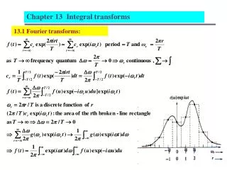
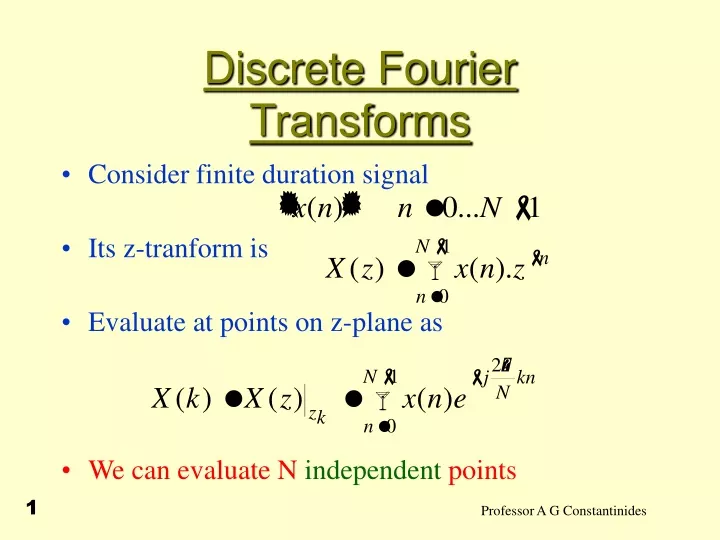
Discrete FourierTransforms • Consider finite duration signal • Its z-tranform is • Evaluate at points on z-plane as • We can evaluate N independent points 1
Discrete FourierTransforms • This is known as the Discrete Fourier Transform (DFT) of • Periodic in k ie • This is as expected since the spectrum is periodic in frequency 2
Discrete FourierTransforms • Multiply both sides of the DFT by • And add over the frequency index k • From which 3
Discrete FourierTransforms • This is the inverse DFT • That is a) the DFT assumes that we deal with periodic signals in the time domain b) Sampling in one domain produces periodic behaviour in the other domain 4
Discrete FourierTransforms • Effectively by knowing • is known everywhere since • or 5
Discrete FourierTransforms • The formula • This is essentially an interpolation and forms the basis of the Frequency Sampling Method for FIR digital filter design 6
Convolution in DFT • Consider the following transform pairs • Define • Find 7
Convolution in DFT • From IDFT • However 8
Convolution in DFT • Or • Thus • This the Circular Convolution 9
Computation of the DFT: The FFT Algorithm • Computation of DFT requires for every sample N multiplications. There are N samples to be computed i.e. time consuming operations. • The Fast Fourier Algorithm:(Decimation in time - DIT, assume even no. of samples) • set 10
FFT • Then DFT of is written • set 11
FFT • ie • Or • Computations of each of summations is now of order ,and thus total computational effort is reduced to . • Continuation of “divide-&-compute” reduces effort to Nlog(N) 12
x(0) X(0) x(4) X(1) x(2) X(2) x(6) X(3) X(4) x(1) x(5) X(5) x(3) X(6) x(7) X(7) a b 8-point FFT • 8-point Signal Flow Diagram 13
N Direct DFT FFT 64 .02 sec .002 sec 512 1 .02 sec 4096 67 .2 32768 1 hr 11 mins 2 262144 3 days 4 hrs 19 FFT times • Time (1 multiplication per microsec) 14
Decimation-in-Time FFT Algorithm • In the basic module two output variables are generated by a weighted combination of two input variables as indicated below where and • Basic computational module is called a butterfly computation 15
Decimation-in-Time FFT Algorithm • Input-output relations of the basic module are: • Substituting in the second equation given above we get 16
Decimation-in-Time FFT Algorithm • Modified butterfly computation requires only one complex multiplication as indicated below • Use of the above modified butterfly computation module reduces the total number of complex multiplications by 50% 17
Decimation-in-Time FFT Algorithm • New flow-graph using the modified butterfly computational module forN = 8 18
Decimation-in-Time FFT Algorithm • Computational complexity can be reduced further by avoiding multiplications by , , , and • The DFT computation algorithm described here also is efficient with regard to memory requirements • Note: Each stage employs the same butterfly computation to compute and from and 19