Download
1 / 57
570 likes | 714 Views
Dark Energy Phenomenology a new parametrization . Je-An Gu 顧哲安 臺灣大學梁次震宇宙學與粒子天文物理學研究中心 Leung Center for Cosmology and Particle Astrophysics (LeCosPA), NTU. Collaborators : Yu-Hsun Lo 羅鈺勳 @ NTHU Qi-Shu Yan 晏啟樹 @ NTHU. 2009/03/19 @ 清華 大學. CONTENTS.

E N D
Dark Energy Phenomenology a new parametrization Je-An Gu顧哲安 臺灣大學梁次震宇宙學與粒子天文物理學研究中心 Leung Center for Cosmology and Particle Astrophysics (LeCosPA), NTU Collaborators : Yu-Hsun Lo 羅鈺勳 @ NTHU Qi-Shu Yan 晏啟樹 @NTHU 2009/03/19 @清華大學
CONTENTS • Introduction (basics, SN, SNAP) • Supernova Data Analysis — Parametrization • A New (model-indep) Parametrization • by Gu, Lo and Yan • Test and Results • Summary
Introduction (Basic Knowledge, SN, SNAP)
Accelerating Expansion Based on FLRW Cosmology (homogeneous & isotropic) Concordance: = 0.73 , M = 0.27
absolute magnitude M luminosity distance dL F: flux (energy/areatime) L: luminosity (energy/time) SN Ia Data:dL(z) [ i.e, dL,i(zi) ] distance modulus redshift z from Supernova Cosmology Project: http://www-supernova.lbl.gov/
Distance Modulus 1998 SCP (Perlmutter et. al.) (can hardly distinguish different models)
Supernova / Acceleration Probe (SNAP) observe ~2000 SNe in 2 years statistical uncertainty mag = 0.15 mag 7% uncertainty in dL sys = 0.02 mag at z =1.5 z= 0.002 mag (negligible) (2366 in our analysis)
Models: Dark Geometryvs. Dark Energy Geometry Matter/Energy ↑ ↑ Dark Geometry Dark Matter / Energy • (from vacuum energy) • Quintessence/Phantom (based on FLRW) Einstein Equations Gμν= 8πGNTμν • Modification of Gravity • Extra Dimensions • Averaging Einstein Equations for an inhomogeneous universe (Non-FLRW)
Supernova Data Analysis — Parametrization / Fitting Formula —
Data vs. Models Observations Data Models Theories Data Analysis mapping out the evolution history (e.g. SNe Ia , BAO) M1 M2 M3 : : : (e.g. 2 fitting) M1 (tracker quint., exponential) M2 (tracker quint., power-law) Quintessence a dynamical scalar field
Reality : Many models survive Observations Data Models Theories Data Analysis mapping out the evolution history (e.g. SNe Ia , BAO) (e.g. 2 fitting) M1(O) M2(O) M3(X) M4(X) M5 (O) M6 (O) : : : Data : : : Shortages: – Tedious. – Distinguish between models ?? – Reality: many models survive. Dark Energy info NOT clear.
Reality : Many models survive • Instead of comparing models and data (thereby ruling out models), Extract information about dark energydirectly from data by invoking model independentparametrizations.
Model-independent Analysis wa wDE(z) 1 -0.5 z -1 0 Linder, PRL, 2003 Riess et al. ApJ, 2007 -1.5 -1 w0 w1 w0 Dark Energy Information Constraints on Parameters Data analyzed by invoking [e.g. wDE(z), DE(z)] Parametrization Fitting Formula in Example Wang & Mukherjee ApJ 650, 2006 w : equation of state, an important quantity characterizing the nature of an energy content. It corresponds to how fast the energy density changes along with the expansion.
Answering questions about Dark Energy Issue How to choose the parametrization? ? • Instead of comparing models and data (thereby ruling out models), Extract information about dark energydirectly from data by invoking model independentparametrizations, thereby answering essential questions about dark energy. “standard parametrization” ?
A New Parametrization (proposed by Gu, Lo, and Yan)
New Parametrization by Gu, Lo & Yan SN Ia Data: dL(z) [ i.e, dL,i(zi) (and errors) ] ( H: Hubble expansion rate ) Assume flat universe. “m”: NR matter – DM & baryons “r”: radiation “x”: dark energy
New Parametrization by Gu, Lo & Yan The density fraction (z)is the very quantity to parametrize. [ instead of x(z) or wx(z) ]
New Parametrization by Gu, Lo & Yan General Features
New Parametrization by Gu, Lo & Yan The lowest-order nontrivial parametrization:
New Parametrization In our analysis, we set by Gu, Lo & Yan i.e., w0 : present value of DE EoS A “amplitude” of the correction x(z) 2 parameters:w0, A
New Parametrization by Gu, Lo & Yan For the present epoch, ignore r(z). Linder
Procedures of Testing Parametrizations Background cosmology [pick a DE Model with wDEth(z)] generate Data w.r.t. present or future observations (Monte Carlo simulation) employ a Fit to the dL(z) or w(z) reconstruct wDEexp’t (z) compare wDEexp’t and wDEth
Gu, Lo & Yan 192 SNe Ia : real data and simulated data 1 overlap consistency Info1 : Black vs. Blue(s) Info2 : Blue vs. Blue no overlap distinguishable real A from 192 SNe Ia w0
Gu, Lo & Yan 192 SNe Ia : real data and simulated data 2 real A from 192 SNe Ia w0 Info1 : Black vs. Blue(s) Info2 : Blue vs. Blue
Gu, Lo & Yan 192 SNe Ia : real data and simulated data 3 real A from 192 SNe Ia w0 Info1 : Black vs. Blue(s) Info2 : Blue vs. Blue
Linder 192 SNe Ia : real data and simulated data 1 from 192 SNe Ia real wa w0 Info1 : Black vs. Blue(s) Info2 : Blue vs. Blue
Linder 192 SNe Ia : real data and simulated data 2 real from 192 SNe Ia wa w0 Info1 : Black vs. Blue(s) Info2 : Blue vs. Blue
Linder 192 SNe Ia : real data and simulated data real 3 from 192 SNe Ia wa w0 Info1 : Black vs. Blue(s) Info2 : Blue vs. Blue
Gu, Lo & Yan Linder A wa w0 w0 From 192 SNe Ia 1 1 real real Info1 : Black vs. Blue(s) Info2 : Blue vs. Blue
Gu, Lo & Yan Linder A wa w0 w0 From 192 SNe Ia 2 2 real real Info1 : Black vs. Blue(s) Info2 : Blue vs. Blue
Gu, Lo & Yan Linder A wa w0 w0 From 192 SNe Ia 3 3 real real Info1 : Black vs. Blue(s) Info2 : Blue vs. Blue
Gu, Lo & Yan from 192 SNe Ia simulated 1 real real data simulated data Info1 : Blue vs. White(s) overlap consistency
Linder from 192 SNe Ia simulated 1 real real data simulated data Info1 : Blue vs. White(s) overlap consistency
Gu, Lo & Yan 2366 simulated SNevs.192 real SNe 1 from 192 real SNe Ia from 2366 simulated SNe Ia A w0
Linder 2366 simulated SNevs.192 real SNe 1 from 192 real SNe Ia from 2366 simulated SNe Ia wa w0
Gu, Lo & Yan 2366 Simulated SN Ia Data 1 A from 2366 simulated SNe Ia w0 Info from comparing nearby contours
Gu, Lo & Yan 2366 Simulated SN Ia Data 2 A from 2366 simulated SNe Ia w0 Info from comparing nearby contours
Gu, Lo & Yan 2366 Simulated SN Ia Data 3 A from 2366 simulated SNe Ia w0 Info from comparing nearby contours
Gu, Lo & Yan 2366 Simulated SN Ia Data 4 A from 2366 simulated SNe Ia w0 Info from comparing nearby contours
Gu, Lo & Yan 2366 Simulated SN Ia Data 5 A from 2366 simulated SNe Ia w0 Info from comparing nearby contours
Linder 2366 Simulated SN Ia Data 1 wa from 2366 simulated SNe Ia w0 Info from comparing nearby contours
Linder 2366 Simulated SN Ia Data 2 wa from 2366 simulated SNe Ia w0 Info from comparing nearby contours
Linder 2366 Simulated SN Ia Data 3 wa from 2366 simulated SNe Ia w0 Info from comparing nearby contours
Linder 2366 Simulated SN Ia Data 4 wa from 2366 simulated SNe Ia w0 Info from comparing nearby contours
Linder 2366 Simulated SN Ia Data 5 wa from 2366 simulated SNe Ia w0 Info from comparing nearby contours
Summary A parametrization (by utilizing Fourier series) is proposed. This parametrization is particularly reasonable and controllable. It is systematical to include more terms and more parameters. Via this parametrization: The current SN Ia data, including 192 SNe, can distinguish between constant-wx models with wx = 0.2 at 1 confidence level. The future SN Ia data, if including 2366 SNe, can distinguish between constant-wx models with wx = 0.05 at 3 confidence level, and the models with wx = 0.1 at 5 confidence level