Download
1 / 38
380 likes | 1.05k Views
OBSERVATION OF ATMOSPHERIC COMPOSITION FROM SPACE. Colette L. Heald ATS 737, October 15, 2008. With material from: Daniel J. Jacob (Harvard), Andreas Richter (Bremen), Cathy Clerbaux (Service d’A é ronomie). WHAT IS THE EFFECT OF ATMOSPHERIC COMPOSITION ON RADIATION?. E + h ν. h ν. h ν.

E N D
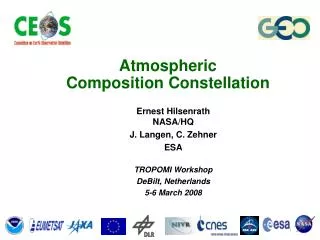
OBSERVATION OF ATMOSPHERIC COMPOSITION FROM SPACE Colette L. Heald ATS 737, October 15, 2008 With material from: Daniel J. Jacob (Harvard), Andreas Richter (Bremen), Cathy Clerbaux (Service d’Aéronomie)
WHAT IS THE EFFECT OF ATMOSPHERIC COMPOSITION ON RADIATION? E + hν hν hν E • OBSERVED RADIATION includes : • Reflection (solar, UV-visible) • Emission (Earth/atmosphere, IR) • Absorption (by gases and particles) • Scattering (by gases and particles) Absorption and emission spectra provide a means of identifying and measuring the composition of the atmosphere. Radiation interacts with gases via: (1) Ionization-dissociation (UV-visible) (2) Electronic transitions (UV-visible) (3) Vibrational transitions (IR) (4) Rotational transitions (far IR and microwave) IR spectra of many molecules is a combination of (3) and (4) • Instead of discrete lines, transitions are observed in a whole wavelength region. • natural line broadening (upper stratosphere, mesosphere) • Doppler broadening (upper atmosphere: > 40 km) • pressure broadening (lower atmosphere: < 40 km) Convolution: Voigt lines
EXAMPLES OF ABSORPTION SPECTRA Hartley band Chappuis band Huggins band
STRATOSPHERIC OZONE HAS BEEN MEASURED FROM SPACE SINCE 1979 Method: UV solar backscatter l1 l2 Ozone layer Scattering by Earth surface and atmosphere Ozone absorption spectrum l1 l2
SATELLITE OBSERVATIONS REVEAL THE MECHANISM FOR POLAR OZONE LOSS AND HELP US TRACK OZONE RECOVERY DU Southern hemisphere ozone column seen from TOMS, October TOMS O3 MLS ClO Polar ozone depletion driven by halocarbon break-down (source of ClO) 1 Dobson Unit (DU) = 0.01 mm O3 STP = 2.69x10¹⁶ molecules cm-2
ATMOSPHERIC COMPOSITION RESEARCH IS NOW MORE DIRECTED TOWARD THE TROPOSPHERE Mesosphere Stratopause Ozone layer Stratosphere Tropopause Troposphere Air quality, climate change, ecosystem issues …but tropospheric composition measurements from space are difficult: optical interferences from water vapor, clouds, aerosols, surface, ozone layer …but tropospheric composition measurements from space are difficult: optical interferences from water vapor, clouds, aerosols, surface, ozone layer
WHY OBSERVE TROPOSPHERIC COMPOSITION FROM SPACE? Global/continuous measurement capability important for range of issues: Monitoring and forecasting of air quality: ozone, aerosols Long-range transport of pollution Monitoring of sources: pollution and greenhouse gases Radiative forcing • solar backscatter • thermal emission • solar occultation • lidar FOUR OBSERVATION METHODS:
SOLAR BACKSCATTER MEASUREMENTS (UV to near-IR) Examples: TOMS, GOME, SCIAMACHY, MODIS, MISR, OMI, OCO absorption l1 l2 z l1 l2 wavelength Retrieved column in scattering atmosphere depends on vertical profile; need chemical transport and radiative transfer models Scattering by Earth surface and by atmosphere concentration • Daytime only • Column only • Interference from stratosphere • sensitivity to lower troposphere • small field of view (nadir) Pros: Cons:
THERMAL EMISSION MEASUREMENTS (IR, mwave) Examples: MLS, IMG, MOPITT, MIPAS, TES, HIRDLS, IASI NADIR VIEW LIMB VIEW elIl(T1) T1 Absorbing gas • versatility (many species) • small field of view (nadir) • vertical profiling Pros: Il(To) To EARTH SURFACE • low S/N in lower troposphere • water vapor interferences • cannot see through clouds Cons:
OCCULTATION MEASUREMENTS (UV to near-IR) Examples: SAGE, POAM, GOMOS “satellite sunrise” Tangent point; retrieve vertical profile of concentrations EARTH • sparse data, limited coverage • upper troposphere only • low horizontal resolution • large signal/noise • vertical profiling Pros: Cons:
LIDAR MEASUREMENTS (UV to near-IR) Examples: LITE, GLAS, CALIPSO Pros: • High vertical resolution Laser pulse • Aerosols only (so far) • Limited coverage Cons: Intensity of return vs. time lag measures vertical profile backscatter by atmosphere EARTH SURFACE
ALL ATMOSPHERIC COMPOSITION DATA SO FAR HAVE BEEN FROM LOW-ELEVATION, SUN-SYNCHRONOUS POLAR ORBITERS • Altitude ~ 1,000 km • Observation at same time of day everywhere • Period ~ 90 min. • Coverage is global but sparse
TROPOSPHERIC COMPOSITION FROM SPACE:platforms, instruments, species
OBSERVING TROPOSPHERIC OZONE AND ITS SOURCES FROM SPACE Nitrogen oxide radicals; NOx = NO + NO2 Sources: combustion, soils, lightning Methane Sources: wetlands, livestock, natural gas Nonmethane VOCs (volatile organic compounds) Sources: vegetation, combustion CO (carbon monoxide) Sources: combustion, VOC oxidation Tropospheric ozone precursors
A NEEDLE IN A HAYSTACK: DERIVING TROPOSPHERIC OZONE • Issues: • high uncertainty • seasonal averages only • does not extend to high latitudes Fishman and Larson, 1987; Fishman et al., 2008
FIRST REMOTE MEASUREMENTS OF CO: MAPS ABOARD THE SPACE SHUTTLE Gas-correlation radiometer (IR: 4.7 m): flew 4 times between 1981 and 1994 APR 1994 OCT 1994 Connors et al., 1999; Reichle et al., 1999
RETRIEVALS IN THE IR: THE STANDARD INVERSE PROBLEM Characteristic absorption features in the IR. Use a known T profile to estimate the constituents INVERSE PROBLEM: solution is not unique! SOLUTION: maximum a posteriori Averaging kernel (A): describes the relative weighting of the ‘true’ mixing ratio (x) at each level to the retrieved value ( ) Typical MOPITT Averaging Kernel
MOPITT: FIRST SATELLITE INSTRUMENT TARGETTING TROPOSPHERIC POLLUTION Spring 2001 MOPITT CO Column CO Column over the NE Pacific in Spring 2001 MOPITT: solid Model: dotted MOPITT – Model Observations used to track transpacific transport of pollution Comparison indicates that emission inventories may be inaccurate Heald et al., 2004
POLLUTION AND BIOMASS BURNING OUTFLOW DURING ICARTT AIRCRAFT MISSION (Jul-Aug 2004) NEAR-REAL-TIME DATA FOR CO COLUMNS ON JULY 18 AIRS GEOS-Chem Model Alaskan fires U.S. pollution Asian pollution Wallace McMillan (UMBC) Turquety et al., 2006
USING MODIS TO MAP FIRESAND MOPITT CO TO OBSERVE EMISSIONS Bottom-up emission inventory (Tg CO) for North American fires in Jul-Aug 2004 From above-ground vegetation From peat 9 Tg CO 18 Tg CO MOPITT CO Summer 2004 GEOS-ChemCO x MOPITT AK with peat burning without peat burning MOPITT data support large peat burning source, pyro-convective injection to upper troposphere Turquety et al., 2006
USING ADJOINTS OF CHEMICAL TRANSPORT MODELS TO INVERT FOR EMISSIONS WITH HIGH RESOLUTION MOPITT daily CO columns (Mar-Apr 2001) Correction to model sources of CO Inverse of atmospheric model A priori emissions from Streets et al. [2003] and Heald et al. [2003] Kopacz et al., 2008
CONSTRAINING NOx AND REACTIVE VOC EMISSIONS USING SOLAR BACKSCATTER MEASUREMENTSOF TROPOSPHERIC NO2 AND FORMALDEHYDE (HCHO) GOME: 320x40 km2 SCIAMACHY: 60x30 km2 OMI: 24x13 km2 Tropospheric NO2 column ~ ENOx Tropospheric HCHO column ~ EVOC ~ 2 km hn (420 nm) BOUNDARY LAYER hn (340 nm) NO2 NO HCHO CO OH hours O3, RO2 hours VOC 1 day HNO3 Emission Deposition Emission VOLATILE ORGANIC COMPOUNDS (VOC) NITROGEN OXIDES (NOx)
DIFFERENTIAL OPTICAL ABSORPTION SPECTROSCOPY Pioneered for stratospheric ozone, used for detection in UV-visible Use multiple wavelengths to characterize optical absorption of a species. determine the amount of absorber along the light path (slant column, s) Scattering by Earth surface and by atmosphere Vertical column: Air mass factor (AMF) depends on the viewing geometry, the scattering properties of the atmosphere, and the vertical distribution of the absorber Or alternate of DOAS: direct fit of GOME backscattered spectrum in 338-356 nm HCHO band Requires an RT model and a CTM Chance et al. [2000]
AMF FORMULATION FOR A SCATTERING ATMOSPHERE what GOME sees GOME sensitivity w(z) HCHO mixing ratio profile S(z) (GEOS-Chem) w(z): GOME sensitivity (“scattering weight”), determined from LIDORT radiative transfer model including clouds and aerosols S(z): normalized mixing ratio (“shape factor”) from GEOS-Chem CTM AMFG: geometric air mass factor (no scatter) AMFG = 2.08 actual AMF = 0.71 Palmer et al., 2001
GEOS-CHEM model (GEIA) GOME CONSTRAINTS ON NOx EMISSIONS Tropospheric NO2 Columns GOME JJA 1997 r = 0.75 bias=5% 1015 molecules cm-2 Martin et al. [2003] Error weighting A priori emissions (GEIA) A posteriori emissions Difference
HIGHER SPATIAL RESOLUTION FROM SCIAMACHY Launched in March 2002 aboard Envisat 60x30 km2 320x40 km2 Potential for finer resolution of sources, but need to account for transport will complicate the inversion
TROPOSPHERIC NO2 FROM OMI: CONSTRAINT ON NOx SOURCES October 2004 K. Folkert Boersma (KNMI)
NOX MEASUREMENTS REVEAL TRENDS IN DOMESTIC EMISSIONS NO2 emissions in US, EU and Japan decline … while emissions growing in China East-Central China Importance of long-term record! Richter et al., 2005; Fishman et al., 2008
FORMALDEHYDE COLUMNS MEASURED BY GOME (JULY 1996) 2.5x10¹⁶ molecules cm-2 2 1.5 1 detection limit 0.5 South Atlantic Anomaly (disregard) 0 -0.5 High HCHO regions reflect VOC emissions from fires, biosphere, human activity
SEASONAL VARIATION OF GOME FORMALDEHYDE COLUMNS reflects seasonal variation of biogenic isoprene emissions GOME GEOS-Chem (GEIA) GOME GEOS-Chem (GEIA) MAR JUL APR AUG SEP MAY JUN OCT Abbot et al., 2003
AEROSOLS FROM SPACE • MIE SCATTERING • scattering on „large“ particles (aerosols, droplets, suspended matter in liquids) • explained by coherent scattering from many individual particles • for spherical particles, Mie scattering can be computed from the refractive index using the Maxwell equations • wavelength of incoming radiation is not changed • angular distribution is changed • depending on , forward scattering is strongly favoured • effectiveness of Mie scattering is proportional to sMie() -1 ... -1.5 • in general, Mie scattering is not polarising Usually in visible Extinction = Scattering + Absorption To retrieve aerosol optical depth need aerosol properties (size distribution, index of refraction). Can use wavelength dependence to get idea of composition/size ISSUE: Need to characterize Rayleigh scattering and surface reflectance (including sun glint) thus easier over oceans (dark surfaces) MODIS MISR • Depending on the ratio of the size of the scattering particle (r) to the wavelength () of the light: • Mie parameter = 2 r / , • different regimes of atmospheric scattering can be distinguished. MULTI-ANGLE: 9 cameras (visible) MULTI-SPECTRAL: 7 bands from 0.4 – 2.1 µm
TRANSPACIFIC TRANSPORT OF ASIAN AEROSOL POLLUTION AS SEEN BY MODIS Detectable sulfate pollution signal correlated with MOPITT CO Heald et al., 2006
MAPPING SURFACE PM2.5 USING MISR (2001 data) MISR AOD (annual mean) Validation with AERONET: R2=0.80 Slope=0.88 Convert AOD to surface PM2.5 using GEOS-CHEM +GOCART scaling factors MISR PM2.5 EPA (FRM+STN) PM2.5 Evaluate against EPA station data: R = 0.78, Slope = 0.91 Liu et al.,2004
NASA AURA SATELLITE (launched July 2004) Aura Direction of motion MLS HIRDLS TES nadir TES limb OMI Polar orbit; four passive instruments observing same air mass within 14 minutes Tropospheric measurement capabilities: • OMI: UV/Vis solar backscatter • NO2, HCHO. ozone, BrO columns • TES: high spectral resolution thermal IR emission • nadir ozone, CO • limb ozone, CO, HNO3 • MLS: microwave emission • limb ozone, CO (upper troposphere) • HIRDLS: high vertical resolution thermal IR emission • ozone in upper troposphere/lower stratosphere
TROPOSPHERIC OZONE OBSERVED FROM SPACE IR emission measurement from TES UV backscatter measurement from GOME GOME JJA 1997 tropospheric columns (Dobson Units) Coincident CO measurements from TES Coincidental observations of CO and O3 with TES allows us to look at ozone production Zhang et al., 2006 Liu et al., 2006
OBSERVING CO2 FROM SPACE:Orbiting Carbon Observatory (OCO) to be launched in 2009 Polar-orbiting solar backscatter instrument, measures CO2 absorption at 1.61 and 2.06 mm, O2 absorption (surface pressure) at 0.76 mm: global mapping of CO2 column mixing ratio with 0.3% precision Pressure (hPa) Averaging kernel (sensitivity) OCO will provide powerful constraints on regional carbon fluxes
LOOKING TOWARD THE FUTURE: GEOSTATIONARY ORBIT • UV-IR sensors would provide continuous high-resolution mapping (~1 km) • on continental scale: boon for air quality monitoring and forecasting NRC Decadal Survey Recommendation: GEO-CAPE in 2013-2016, with Aura-like GACM in 2016-2020 (also ACE for aerosols 2013-2016) NRC, 2007