Download

1 / 51
510 likes | 670 Views
The Demand for Labor. Hwei-Lin Chuang, Ph.D. 2014/03/11. 2014-2016 數位內容產業人才需求調查報告摘要. 產業發展趨勢對人才需求的影響 行動化: 據資策會 FIND 估計,預期 2018 年,平板電腦將是繼上網人口、社群人口、智慧型手機,為第四個具備千萬用戶的智慧終端。產業需要更多行動開發人才 (App 程式開發、 UI/UX 設計人才 ) 。

E N D
The Demand for Labor Hwei-Lin Chuang, Ph.D. 2014/03/11
2014-2016數位內容產業人才需求調查報告摘要 • 產業發展趨勢對人才需求的影響 • 行動化:據資策會FIND估計,預期2018年,平板電腦將是繼上網人口、社群人口、智慧型手機,為第四個具備千萬用戶的智慧終端。產業需要更多行動開發人才(App程式開發、UI/UX設計人才) 。 • 匯流化:隨4G服務上線,未來4年臺灣將進入行動大寬頻時代,核心及關聯產業之間的界線越來越模糊,隨著商業模式混搭並持續創新,未來如何整合運用在內容開發及市場喜好掌握等,是國內業者最大的瓶頸。產業需要培育更多具備跨界整合能力的人才以因應產業匯流之趨勢。 • 國際化:臺灣數位內容產業市場規模小,國際化擴張是必要手段,國際市場目前在中國大陸遭遇不少進入障礙,未來國際市場可聚焦策略性重點國家如日本及東協國家市場,產業需要更多行銷(懂當地市場)人才、在職人才需提升國際化/語言能力。 資料來源:經濟部工業局2014-2016數位內容產業專業人才需求調查(2013) 資料整理:繆淑蓉/工研院產業學院副管理師
表一 數位內容產業專業人才關鍵職缺需求調查結果表 資料來源:經濟部工業局2014-2016數位內容產業專業人才需求調查(2013) 資料整理:繆淑蓉/工研院產業學院副管理師
表一(續)數位內容產業專業人才關鍵職缺需求調查結果表表一(續)數位內容產業專業人才關鍵職缺需求調查結果表
跨界新人才 等你卡位! 文/2013年1月號數位時代採訪.撰文/趙郁竹 攝影/賀大新 插畫繪製/JV. Huang • 回想一下,五年前第一支iPhone剛問世,沒有人想像得到App帶來的新經濟浪潮,但現在,每家企業都想開發App,讓Objective-C程式工程師成為市場搶手貨。從電腦、網路到現在的雲端,未來人與人、人與機器、機器與機器,都將產生全面連結,數位匯流和大資料(Big Data)應用起飛,推動整個商業社會的轉型。 • 未來需求一:跨界人才 • 過去台灣企業重視的特質是服從、盡職、單一領域的專業,「但未來最有競爭力的人才是熱情、創新,而且具備跨領域專業能力,」本土工業電腦大廠研華科技總經理何春盛指出。例如遠距照護、健康雲、智慧交通……,都是政府正大力建設的科技應用,這些都需要懂科技又懂產業知識的跨界人才。 • 未來需求二:國際化人才 • 擁有國際化能力,走到哪裡都吃香。「IBM徵才最重視兩件事:專業能力和國際觀,」IBM人力資源部處長林雅莉說,國際企業希望員工不畫地自限,走到哪都能工作。 • 但如何在面試官前呈現自己的國際化能力?首先當然英文能力是基本功,但所謂國際觀不是只有語言能力,林雅莉建議,年輕人從在學時就應開放心胸、自我練習,例如邀請不同國家、不同文化的人共學。 • 根據1111人力銀行統計資料,2011年資訊/科技產業一年以下經驗新鮮人的平均薪資為3萬1305元,比2010年增加了1352元。若單看工程研發職務,新鮮人平均起薪更達3萬5103元。「22K到15K」之說讓許多人心惶惶,但簡立峰、張明正都認為,年輕人的未來其實沒有那麼糟,只要掌握跨領域、國際化能力,再加上一點樂觀和自信,機會自然會到眼前。
眼界的遠近,決定你的機會─台灣軟體人才的機會與挑戰眼界的遠近,決定你的機會─台灣軟體人才的機會與挑戰 文/2014年2月號數位時代撰文者/陳芷鈴 • 在台灣,軟體相關科系向來是升學大熱門,每一屆畢業生投入軟體業者也不在少數,但為何台灣缺乏軟體人才的聲浪依舊不斷?全球最大的國際性人力資源服務公司藝珂人事顧問東北亞區執行長陳玉芬以及協理劉小筠,從全球人才招募者的角度,分享台灣軟體人才的機會與挑戰。 • Q近年在找軟體人才有沒有感受到一些新需求或新趨勢? • 劉小筠:現在所有科技業都講求創新,很多人才需求可能昨天沒有,但今天就產生出來。軟體人才可能有技術開發、技術應用或是將這些技術轉成可使用的程式設計工程師等,其實整個市場是在擴大的,有傳統需要的軟體人才,也有因應新技術或新消費市場需求所產生的職缺,比如像4G,就可能產生跟通訊、大數據、雲端運算等相關的軟體人才需求。這些趨勢會持續不斷發展,未來如果能發展個三十年,我們目前可能才走完第一個十年,還有很多未知的東西。 • Q 走出去學習的確是能夠帶回創新,但就我們台灣產業來說,是否也有一些軟體人才的發展空間呢? • 陳玉芬:我們是鼓勵candidate(職位候選人)多去爭取一些國際性的計畫,他們也可以在家完成工作啊!不要只想找離家近的工作,眼光放遠一點,你可以試著談判,談看看可不可以在家工作,讓你的工作管道可以廣一點,這樣子的眼界對我們的產業來說也是好的。
事業單位預計:103年4月底人力需求較1月底淨增加36.7千人事業單位預計:103年4月底人力需求較1月底淨增加36.7千人 勞動部103.03.04 新聞稿 • 為了解民國103年4月底就業市場人力需求情況,勞動部於103年1月13~29日針對員工規模30人以上的事業單位辦理「103年第1次人力需求調查」,總計回收有效樣本3,015家,調查統計結果摘述如下: • 事業單位預計103年4月底人力需求較1月底淨增加36.7千人,主因全球復甦步調穩定、先進國家景氣明顯回溫,內、外需皆漸有支撐,廠商增僱員工意願持續提升。 • 按行業別觀察,淨增加僱用人力的行業以製造業淨增19.4千人較為明顯,其次為批發零售業淨增5.0千人、住宿及餐飲業淨增2.9千人 • 按職類別觀察,以技術員及助理專業人員淨增加11.4千人、技藝/機械設備操作及組裝人員淨增加10.3千人最多 • 整體來看,增加僱用人力的原因以「需求市場擴大(含設備或部門擴充)」及「退離者補充」為主。
表二 事業單位預計103年4月底較1月底僱用人力增減情形
表三 eJob全國就業e網2014/01/01~2014/03/07熱門職缺統計表
表三 eJob全國就業e網2014/01/01~2014/03/07熱門職缺統計表(續)
表三 eJob全國就業e網2014/01/01~2014/03/07熱門職缺統計表(續) 資料來源:eJob全國就業e網 http://www.ejob.gov.tw/about/HotJobList.aspx
THE DEMAND FOR LABOR • The demand for labor is a derived demand. Employer’s demand for labor is a function of the characteristics of demand in the product market. It is also a function of the characteristics of the production process.
Introduction • Firms hire workers because consumers want to purchase a variety of goods and services. • Demand for workers is derived from the wants and desires of consumers. • Central questions: how many workers are hired and what are they paid?
Two important features of the demand for labor: • It can be shown theoretically and empirically that labor demand curves slope downward. • The quantity of labor demanded has varying degrees of responsiveness to changes in the wage.
When the demand for labor is analyzed, two sets of distinctions are made: • Demand by firm v.s. the demand curves for an entire market. Note: Firm and market labor demand curves have different properties although both slope downward. • The time period for which the demand curve is drawn. Short Run: A period over which a firm’s capital stock is fixed. Long Run: A period over which a firm is free to vary all factors of production.
A Simple Model of Labor Demand Assumptions: (1) Employers seek to maximize profit. (2) Firms employ two homogeneous factors of production, employee-hours (E) and capital (K), in their production of goods and services. Their production function can be written as: Q = f (E, K) (3) Hourly wage cost is the only cost of labor. Note: We ignore hiring, training cost and fringe- benefit costs for the time being. (4) Both a firm’s labor market and its product market are competitive.
The Firm’s Production Function • Describes the technology that the firm uses to produce goods and services. • The firm’s output can be produced by a variety of capital–labor combinations. • The marginal product of labor is the change in output resulting from hiring an additional worker, holding constant the quantities of other inputs. • The marginal product of capital is the change in output resulting from hiring one additional unit of capital, holding constant the quantities of other inputs.
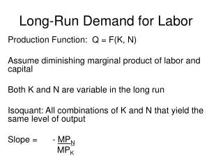
1. Short-Run Demand for Labor by Firms Defn. Marginal Product of Labor: The change in output resulting from hiring an additional worker, holding constant the quantities of all other input. Output Output 140 Average Product 25 120 20 100 15 80 60 10 40 Marginal Product 5 20 0 2 4 6 8 10 2 4 6 8 10 0 Number of workers Number of workers The Total Product, the Marginal Product, and the Average Product Curves
Defn. Law of Diminishing Returns: Eventually each additional increment of labor produces progressively smaller increments of output. Defn. Value of the Marginal Product (VMP): The dollar values of the additional output produced by an additional worker. VMP = P ×MPE
The profits are maximized by the competitive firm when the value of marginal product of labor is just equal to its marginal cost. Dollars 38 VAPE 22 VMPE 0 1 4 8 Number of Workers The Firm’s Hiring Decision in the Short Run
Profit-Maximizing condition: Labor should be hired until its marginal product equals the real wage. i.e., MPE=W/P The firm’s demand for labor in the short run is equivalent to the downward-sloping segment of its marginal product of labor schedule. Note: The downward-sloping nature of the short-run labor demand curve is based on an assumption that MPE declines as employment is increased.
Short Run Hiring Decision • Value of Marginal Product (VMP) is the marginal product of labor times the dollar value of the output. • VMP indicates the dollar benefit derived from hiring an additional worker, holding capital constant. • Value of Average Product is the dollar value of output per worker.
Elasticity of Labor Demand We measure the responsiveness of labor demand to changes in the wage rate by using an elasticity. The short-run elasticity of labor demand, δSR, is defined as the percentage change in short-run employment resulting from a 1 percent change in the wage: δSR = (%△ESR)/ (%△w) Since the labor demand curves slope downward, an increase in the wage rate will cause employment to decrease; the (own-wage) elasticity of demand is a negative number.
Note: |δSR | > 1: a 1% increase in wage will lead to an employment decline of greater than 1% → elastic demand curve |δSR | < 1: a 1% increase in wage will lead to a proportionately smaller decline in employment → inelastic demand curve Elastic demand: aggregate earnings↓ when w↑ Inelastic demand: aggregate earnings↑ when w↑ W D2 D1 W’ D1: elastic demand D2: inelastic demand W E E1 E1’ E2’ E2
2. Market Demand Curve A market demand curve is just the summation of the labor demanded by all firms in a particular labor market at each level of the real wage. Note: When aggregating labor demand to the market level, product price can no longer be taken as given, and the aggregation is no longer a simple summation. However, the market demand curves drawn against money wages, like those drawn as functions of real wages, slope downward.
金融相關產業受僱員工概況 (101)(單位:人、元)金融相關產業受僱員工概況 (101)(單位:人、元) 資料來源:勞動部資料庫 http://www.mol.gov.tw/cgi-bin/siteMaker/SM_theme?page=450f92d3
金融相關產業受僱員工概況(續)(101)(單位:人、元)金融相關產業受僱員工概況(續)(101)(單位:人、元)
3. Long-Run Demand for Labor by Firms In the long run, employers are free to vary their capital stock as well as the number of workers they employ. • Profit Maximization’s Dual Problem – Cost Minimization Defn. Isoquant: An isoquant describes the possible combination of labor and capital which produce the same level of output. Defn.The Marginal Rate of Technical Substitution: The slope of an isoquant is the negative of the ratio of marginal products. The absolute value of the slope of an isoquant is called the marginal rate of technical substitution. Defn. Isocost: The isocost line gives the menu of different combinations of labor and capital which are equally costly.
A profit-maximizing firm that is producing q0 units of output wants to produce these units at the lowest possible cost. →The firm chooses the combination of labor and capital where the isocost is tangent to the isoquant. i.e., MPE/MPK = w/r →Cost-minimization requires that the marginal rate of technical substitution equal the ratio of prices.
Capital Note: To be minimizing cost, the cost of producing an extra unit of output by adding only labor must equal the cost of producing that extra unit by employing only additional capital. i.e., C1/r A C0/r P 175 B MPE/w = MPK/ r 0 100 Employment The Firm’s Optimal Combination of Inputs
Cost Minimization • Profit maximization implies cost minimization. • The firm chooses the least-cost combination of capital and labor. • This least-cost choice is where the isocost line is tangent to the isoquant. • Marginal rate of substitution equals the ratio of input prices, w / r, at the least-cost choice.
Long Run Demand for Labor • When the wage drops, two effects arise. • The firm takes advantage of the lower price of labor by expanding production (the scale effect). • The firm takes advantage of the wage change by rearranging its mix of inputs even if holding output constant (the substitution effect)
The Effect of Change in w • Increase in w: • Substitution Effect • As w increase, labor cost rises, and more capital and less labor are used in the production process. • (2) Scale effect • The new-profit-maximizing level of production will be less. How much less cannot be determined unless we know something about the product demand curve.
Both the substitution effect and the scale effect work in the same direction. So these effects lead us to assert that the long-run demand curve for labor slopes downward. Note: In general, if a firm is seeking to minimize costs, in the long run it should employ all inputs up until the point that the marginal cost of producing a unit of output is the same regardless of which input is used.
Capital C0/r R P 75 q0 Wage is w1 Wage is w0 25 40 The Impact of a Wage ReductionHolding Costs Constant A wage reduction flattens the isocost curve. If the firm were to hold the initial cost outlay constant at C0 dollars, the isocost would rotate around C0 and the firm would move from point P to point R. A profit-maximizing firm, however, will not generally want to hold the cost outlay constant when the wage changes. q0
Dollars Capital MC0 MC1 R p P 150 100 100 150 Employment Output 25 50 THE IMPACT OF A WAGE REDUCTION ON THE OUTPUT AND EMPLOYMENT OF A PROFIT-MAXIMIZING FIRM • A wage cut reduces the marginal cost of production and encourages the firm to expand (from producing 100 to 150 units). • The firm moves from point P to point R, increasing the number of workers hired from 25 to 50.
Capital D C1/r Q C0/r R P 200 D 100 Wage is w1 Wage is w0 50 40 25 Employment Substitution and Scale Effects A wage cut generates substitution and scale effects. The scale effect (from P to Q) encourages the firm to expand, increasing the firm’s employment. The substitution effect (from Q to R) encourages the firm to use a more labor-intensive method of production, further increasing employment.
Two Special Cases of Isoquants Capital and labor are perfect substitutes if the isoquant is linear (so that two workers can always be substituted for one machine). The two inputs are perfect complements if the isoquant is right-angled. The firm then gets the same output when it hires 5 machines and 20 workers as when it hires 5 machines and 25 workers.
Elasticity of Substitution • The elasticity of substitution is the percentage change in the capital to labor ratio given a percentage change in the price ratio (wages to real interest). • Formula: %∆(K/L) %∆(w/r). • Interpret a particular elasticity of substitution number as the percentage change in the capital–labor ratio given a 1% change in the relative price of labor to capital
Elasticity of Substitution • Example: If the elasticity of substitution is 5, then a 10% increase in the ratio of wages to the price of capital would result in the firm increasing its capital-to-labor ratio by 50%.
4. Marshall’s Rules of Derived Demand (The Hicks-Marshall Law of Derived Demand) The factors that influence own-wage elasticity can be summarized by the four “Hicks-Marshall Laws of Derived Demand.” These laws assert that, other things equal, the own-wage elasticity of demand for a category of labor is high under the following conditions:
When the price elasticity of demand for the product being produced high; • When other factors of production can be easily substituted for the category of labor; • When the supply of other factors of production is highly elastic; • When the cost of employing the category of labor is a large share of the total cost of production. Note: (1), (2) and (3) can be shown to always hold. There are conditions, however, under which the final law does not hold.
(1) Demand for the Final Product The greater the price elasticity of demand for the final product, the larger will be the decline in output associated with a given increase in price and the greater the decrease in output, the greater the loss in employment (other things equal). Thus the greater the elasticity of demand for the product, the greater the elasticity of demand for labor will be.
(2) SUBSTITUTABILITY OF OTHER FACTORS Other things equal, the easier it is to substitute other factors in production, the higher the wage elasticity of demand will be. Note: (1) Sometimes collectively bargained or legislated restrictions make the demand for labor less elastic by reducing substitutability (not technically). (2) Substitution possibility that are not feasible in the short run may well become feasible over longer periods of time, when employers are free to vary their capital stock. → The demand for labor is more elastic in the longer run than in the short run.
(3) The supply of Other Factors As the wage rate increased and employers attempted to substitute other factors of production for labor, the prices of these inputs were bid up substantially. Such a price increase would dampen firm’s appetites for capital and thus limit the substitution of capital for labor. Note: Prices of other inputs are less likely to be bid up in the long run than in the short run. → Demand for labor will be more elastic in the long run.
(4) The Share of Labor in Total Costs The greater the category’s share in total costs, the higher the wage elasticity of demand will tend to be. If the share of labor cost is large, cost increase due to wage increase is larger. The employer would have to increase their product prices by more, output and hence employment would fall more. Note: This law, relating a smaller labor share with a less-elastic demand curve, holds only when it is easier for customers to substitute among final products than it is for employers to substitute capital for labor.
Factor Demands when thereare Several Inputs • There are many different inputs. • Skilled and unskilled labor • Old and young • Old and new machines • Cross-elasticity of factor demand. • %∆Di%∆wj • If cross-elasticity is positive, the two inputs are said to be substitutes in production.
Price of input i Price of input i D0 D1 D0 D1 Employment of input i Employment of input i THE DEMAND CURVE FOR A FACTOR OF PRODUCTION IS AFFECTED BY THE PRICES OF OTHER INPUTS (a) (b) The labor demand curve for input i shifts when the price of another input changes. (a) If the price of a substitutable input rises, the demand curve for input i shifts up. (b) If the price of a complement rises, the demand curve for input i shifts down.
THE CROSS-WAGE ELASTICITY OF DEMAND The elasticity of demand for input j with respect to the price of input k is the percentage change in the demand for input j induced by 1 percent change in the price of input k. i.e., δjk= %△Ej / %△Wk δjk= %△Ek / %△Wj
If the cross elasticities are positive (with an increase in the price of one increasing the demand for the other) the two are said to be gross substitutes. If the cross elasticities are negative (and increase in the price of one reduces the demand for the other), the two are said to be gross complements. Note: Whether two inputs are gross substitutes or gross complements depends on both the production function and the demand conditions. → Knowing that two groups are substitutes in production is not sufficient to tell us whether they are gross substitutes or gross complements.