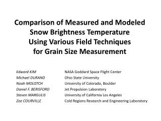
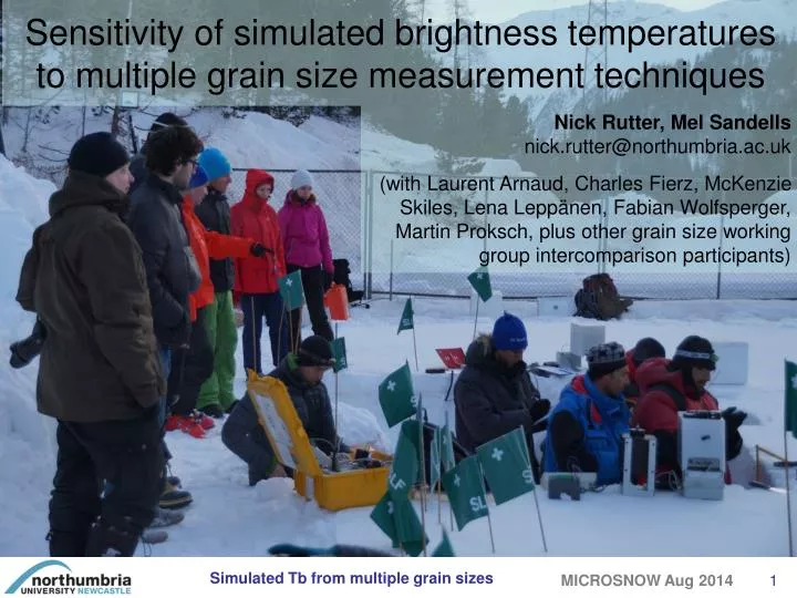
Sensitivity of simulated brightness temperatures to multiple grain size measurement techniques

1. Sensitivity of simulated brightness temperatures to multiple grain size measurement techniques Nick Rutter, Mel Sandells nick.rutter@northumbria.ac.uk (with Laurent Arnaud, Charles Fierz, McKenzie Skiles, Lena Leppänen, Fabian Wolfsperger, Martin Proksch, plus other grain size working group intercomparison participants) Simulated Tb from multiple grain sizes

2. Passive microwave • Only current operational satellite sensors for snow and 30+ year legacy • Optimal configurations of active microwave satellites for snow may be some way off (CoReH20) • Satellites providing a stand alone product? • Global: AMSR-E snow depth 22 cm RMSE, from ~250 WMO stations (Kelly 2009) • Geographically specific improvements: Tundra (Derksen et al. 2010) • Satellites as part of data assimilation product e.g. GlobSnow? • 1-layer emission model (HUT), recognizing grain size as the most sensitive parameter • HUT inverts satellite Tb and known depth to estimate grain size -> grain size spatially interpolated to produce Tb estimates -> minimization of cost function -> maps of assimilated SWE • Current lack of faith in snow depth & mass products by other communities, e.g. not used in LSM benchmarking of NCAR models (David Lawrence, GWEX 2014) Can reduction in uncertainty of snow microstructure measurements improve evaluation of snow emission models? Rationale

3. Aim: quantify variability in brightness temperatures (Tb) simulated by the HUT-ML microwave emission model using different grain size measurements • Unprecedented opportunity to get a wide range of snow grain size values of the same snowpack using different measurement methods • ~19 different instruments participated in the workshop, some with more than one grain size metric. By July 2014 seven QC’d data sets were available from six instruments: • Visual: TRAD (Fierz) • Optical: FCP (Skiles) • SSA: • ASP (Arnaud), • FCP (Skiles), • ICE (Leppanen), • INF (Wolfsperger), • SMP (Proksch). Experimental overview : Measurements

4. Aim: quantify variability in brightness temperatures (Tb) simulated by the HUT-ML microwave emission model using different grain size measurements • Unprecedented opportunity to get a wide range of snow grain size values of the same snowpack using different measurement methods • ~19 different instruments participated in the workshop, some with more than one grain size metric. By July 2014 seven QC’d data sets were available from six instruments: • Visual: TRAD (Fierz) • Optical: FCP (Skiles) • SSA: • ASP (Arnaud), • FCP (Skiles), • ICE (Leppanen), • INF (Wolfsperger), • SMP (Proksch). Experimental overview : Measurements

5. Aim: quantify variability in brightness temperatures (Tb) simulated by the HUT-ML microwave emission model using different grain size measurements • Unprecedented opportunity to get a wide range of snow grain size values of the same snowpack using different measurement methods • ~19 different instruments participated in the workshop, some with more than one grain size metric. By July 2014 seven QC’d data sets were available from six instruments: • Visual: TRAD (Fierz) • Optical: FCP (Skiles) • SSA: • ASP (Arnaud), • FCP (Skiles), • ICE (Leppanen), • INF (Wolfsperger), • SMP (Proksch). Experimental overview : Measurements

6. Aim: quantify variability in brightness temperatures (Tb) simulated by the HUT-ML microwave emission model using different grain size measurements • Unprecedented opportunity to get a wide range of snow grain size values of the same snowpack using different measurement methods • ~19 different instruments participated in the workshop, some with more than one grain size metric. By July 2014 seven QC’d data sets were available from six instruments: • Visual: TRAD (Fierz) • Optical: FCP (Skiles) • SSA: • ASP (Arnaud), • FCP (Skiles), • ICE (Leppanen), • INF (Wolfsperger), • SMP (Proksch). Experimental overview : Measurements

7. Aim: quantify variability in brightness temperatures (Tb) simulated by the HUT-ML microwave emission model using different grain size measurements • Unprecedented opportunity to get a wide range of snow grain size values of the same snowpack using different measurement methods • ~19 different instruments participated in the workshop, some with more than one grain size metric. By July 2014 seven QC’d data sets were available from six instruments: • Visual: TRAD (Fierz) • Optical: FCP (Skiles) • SSA: • ASP (Arnaud), • FCP (Skiles), • ICE (Leppanen), • INF (Wolfsperger), • SMP (Proksch). Experimental overview : Measurements

8. Aim: quantify variability in brightness temperatures (Tb) simulated by the HUT-ML microwave emission model using different grain size measurements • Unprecedented opportunity to get a wide range of snow grain size values of the same snowpack using different measurement methods • ~19 different instruments participated in the workshop, some with more than one grain size metric. By July 2014 seven QC’d data sets were available from six instruments: • Visual: TRAD (Fierz) • Optical: FCP (Skiles) • SSA: • ASP (Arnaud), • FCP (Skiles), • ICE (Leppanen), • INF (Wolfsperger), • SMP (Proksch). Experimental overview : Measurements

9. Model inputs (1-D profiles of stratigraphy, density, temperature and ‘grain size’) • Stratigraphy, layer identification (ice, crusts, grain type) in pit MA1 (Fierz), • Density measurements (n = 3) so….used density in pit MA3 (< 2 m away), which had 3 cm vertical resolution using 100 cm^3 cutter (Proksch) (n = 44) • Temperature (2 to 10 cm vertical resolution) • Substrate was a frozen clay tennis court Experimental methods: Measurements

10. Thanks to Charles Fierz WSL Institute for Snow and Avalanche Research SLF

11. Data: Density profiles

12. Grain size measurements were averaged within stratigraphic layers • Cubic interpolation used to determine temperature and grain size for thin layers • Model parameters: Roughness = 0, epsilon = 6-j; Angle = 53 deg, Freq/Pol: 19V 19H 37V 37H • Effective grain diameter determine from visual / optical and SSA: • Visual (d obs) and optical to effective grain size (Deff):following Kontu and Pulliainen (2010) • SSA (per mass of ice) to effective grain size following Gallet et al. (2009) and Montpetit et al. (2012): • SMP derives SSA from correlation length (pc) following Debye et al. (1957): Experimental methods: HUT-ML emission model

13. For each combination of frequency and polarisation: three extinction coefficients: • Hallikainen et al. (1987), from snow in southern Finland: • Kontu and Pulliainen (2010), optimized for deeper and denser snow with larger grain sizes than taiga snow: • Roy et al. (2004), to account for multiple scattering by densely packed ice particles where γ and δ are 2 ± 1 and 0.20 ± 0.04 respectively: Experimental methods: HUT-ML emission model

14. Visual (TRAD) lowest Tb • SSA reasonably similar with exception of SMP ( a bit lower) • ICE and ASP very similar (should be as same techniques) • Optical FCS similar to SSA FCS Results

15. Conclusions • Quantified spread in Tb from a snow emission model from eight independent grain size measurements (a first with this many simultaneous measurements?) • Improvement on sensitivity analysis using synthetic grain size data (constrains relative grain size differences between stratigraphic layers) • Despite looking at the same snow in the most controlled circumstances as possible, measurements techniques propagate a 6-82 K spread in estimated Tb • With the caveat that is just a quick pilot study which needs more thorough work, there is clearly a challenge ahead. How might a follow-up experiment meet this challenge? Results & Conclusion

16. Need to know more about the substrate • Completely frozen? • Percentage interstitial liquid water content? • Soil texture? Organics? • Groups currently working on this for soil moisture and freeze-thaw • More snowpack heteorgeneity? • St Mortiz homogeneity ideal for measurement inter-comparison (tennis court, wind-sheltered) • Lacking in snow grain types (e.g. depth hoar and wind slab) that are representative of shallow sub-Arctic to high-Arctic snowpacks (< 120-150 mm SWE saturation levels) • More applicable to satellite remote sensing & assimilation products? • Can we conduct a similar experiment to St Moritz • in Arctic or sub-Arctic snowpacks ? Future experiment?

17. Capability: independent Tb measurements for model evaluation using portable ground-based (sled-mounted) radiometers There’s extra capacity within working group to provide redundancy Future experiment?

18. Capability: identify spatial variability in stratigraphic layer boundaries at sub-cm resolution in shallow (< 1m) snowpacks Rutter et al. (2014) Domine et al. (2012) Future experiment?

19. Capability: spatially interpolate 1-D profiles of measurements throughout horizontal layers Watts et al. (in prep.) Future experiment?

20. Large 50 m extents: • Lengths scales of layer thickness & layer properties, • Roughness of layer boundaries, • Distributions of layer properties (tails!) as model inputs. Future experiment?

21. Physical snow model with full range of snow process representations (e.g. Essery et al., 2013) • Multiple grain size measurement techniques (X-ray tomography, plus multiple SSA, Pc, Optical) • Seasonal grain size evaluation data • Emission model interchangeability incorporating easy: • Conversion between grain size metrics (SSA, Pc, Dobs, Opt) • Field data & snow model output to emission model initialization (HUT, DMRT, MEMLS) • Long term, high quality meteorological data & logistical support in Arctic environment with cost-efficient accessibility • Goal: to allow all modelling groups to evaluate uncertainties, algorithms and process representations in the estimation of Tb Wish list

22. Extra Slides

23. Differences in Tb using Fierz low resolution densities (n=3) and Proksch high resolution densities (n=44)

25. Data: Snowpit measurements