Download
1 / 35
350 likes | 505 Views
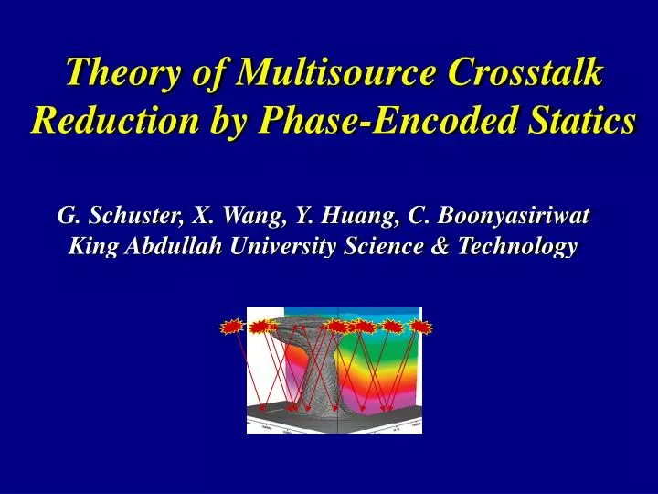
Theory of Multisource Crosstalk Reduction by Phase-Encoded Statics. G. Schuster, X. Wang, Y. Huang, C. Boonyasiriwat King Abdullah University Science & Technology. Outline. Seismic Experiment:. L m = d. 1. 1. L m = d. 2. 2. L m = d. N. N.

E N D
Theory of Multisource Crosstalk Reduction by Phase-Encoded Statics G. Schuster, X. Wang, Y. Huang, C. Boonyasiriwat King Abdullah University Science & Technology
Outline Seismic Experiment: Lm = d 1 1 Lm = d 2 2 Lm = d . . N N . 2. Standard vs Phase Encoded Least Squares Soln. L d 3. Theory Noise Reduction ]m = [N d + N d ] vs [ N L + N L 1 1 m = L d 2 2 2 2 1 1 1 1 2 2 4. Summmary and Road Ahead
Gulf of Mexico Seismic Survey 4 d Predicted data Observed data 1 Goal: Solve overdetermined System of equations for m Time (s) Lm = d 1 1 Problem: Expensive, one migration/shot gather 0 Lm = d 6 X (km) 2 2 Solution:Supergather migration Lm = d . . N N . m
Seismic Inverse Problem 2 Soln: min || Lm-d || migration waveform inversion -1 T T m = [L L] L d T L d Given: d= Lm Find: m(x,y,z)
Computational Challenges -1 T T m = [L L] L d Given: d= Lm Find: d > 10 13 words 7 m > 10 3 20x20x10 km unknown velocity values 4 dx=1 m # time steps ~ 10 4 # shots > 10 Total = 15 10
Brief History Multisource Phase Encoded Imaging Migration Romero, Ghiglia, Ober, & Morton, Geophysics, (2000) Waveform Inversion and Least Squares Migration Krebs, Anderson, Hinkley, Neelamani, Lee, Baumstein, Lacasse, SEG, (2009) Virieux and Operto, EAGE, (2009) Dai and Schuster, SEG, (2009) Biondi et al., SEG, (2009)
Outline Seismic Experiment: Lm = d 1 1 Lm = d 2 2 Lm = d . . N N . 2. Standard vs Phase Encoded Least Squares Soln. L d 3. Theory Noise Reduction ]m = [N d + N d ] vs [ N L + N L 1 1 m = L d 2 2 2 2 1 1 1 1 2 2 4. Summmary and Road Ahead
Conventional Least Squares Solution: L= & d = L d 1 1 L d Given: Lm=d 2 2 In general, huge dimension matrix Find: m s.t. min||Lm-d|| 2 Solution: m = [L L] L d -1 T T or if L is too big m = m – aL (Lm - d) (k+1) (k) (k) T (k) = m – aL (L m - d ) (k) (k) [ ] T + L (L m - d ) T 1 1 1 2 2 2 Note: subscripts agree Problem: L is too big for IO bound hardware
Conventional Least Squares Solution: L= & d = L d 1 1 L d Given: Lm=d 2 2 In general, huge dimension matrix Find: m s.t. min||Lm-d|| 2 Solution: m = [L L] L d -1 T T m = m – aL (Lm - d) (k+1) (k) (k) T (k) = m – aL (L m - d ) (k) (k) [ ] T + L (L m - d ) T 1 1 1 2 2 2 Problem: Expensive, FD solve/CSG Solution: Blend+encode Data Problem: L is too big for IO bound hardware
Blending+Phase Encoding Blending Blending Phase Phase 1 d d d Lm= Lm= Lm= 1 1 3 2 2 3 Encoded supergather O(1/S) cost! Encoding Matrix d = N d + N d + N d in w domain 1 1 2 3 2 3 Encoded supergather modeler L = NL + N L + NL m [ ]m 1 2 3 1 2 3 e iwt
Blended Phase-Encoded Least Squares Solution L =&d = N d + N d N L + N L 1 2 1 1 1 2 2 2 Given: Lm=d In general, SMALL dimension matrix Find: m s.t. min||Lm-d|| 2 Solution: m = [LL] Ld -1 T T or if L is too big m = m – aL (Lm - d) T (k+1) (k+1) (k) (k) (k) (k) (k) = m – aL (L m - d ) (k) (k) (k) (k) [ (k) (k) ] (k) (k) T + L (L m - d ) T (k) Iterations are proxy For ensemble averaging 1 1 1 2 2 2 + Crosstalk * * (k) + L N N (L m - d ) (k) (k) (k) (k) (k) (k) T L N N (L m - d ) (k) T + (k) (k) (k) (k) 2 1 2 1 1 1 2 2 2 1
Outline Seismic Experiment: Lm = d 1 1 Lm = d 2 2 Lm = d . . N N . 2. Standard vs Phase Encoded Least Squares Soln. L d 3. Theory Noise Reduction ]m = [N d + N d ] vs [ N L + N L 1 1 m = L d 2 2 2 2 1 1 1 1 2 2 4. Summary
Ensemble Average of Crosstalk Term With Random Time Shifts e -iwt 2 + Crosstalk: Noise = e e e iw(t - t ) iwt <Noise>: < > -iwt < > = < > 1 1 2 2 Gaussian PDF 2 e iw(t - t ) -.25 s (t - t ) e = 1 2 1 2 -2 2 Crosstalk term decreases with increasing w and s -s w e ~ dtdt 1 2 * * * L N N (L m - d ) N N T L N N (L m - d ) T 1 1 2 1 2 1 1 1 2 2 2 2 1
Crosstalk Prediction Formula ~ X = O( ) 2 2 e -s w Pt. Scatt. Stand. Mig. Pt. Scatt.. Mig. of Supergathers. Depth s = .01 s X Offset Pt. Scatt.. Mig. of Supergathers. Pt. Scatt.. Mig. of Supergathers. s = .05 s s = .1 s .01 1.0 s L (L m - d ) + L (L m - d ) T T 2 1 1 2 1 2
sgn(t ) Ensemble Average of Crosstalk Term With Random Polarity sgn(t) + Crosstalk: Noise < > = < > sgn(t ) sgn(t ) <Noise>: = 0 1 2 Conclusion: Random polarity better than random time shifts Further Analysis: Variance of the crosstalk noise says that random polarity & random time shifts has ½ less than variance of polarity alone ( ) 2 < > * * * * L N N (L m - d ) N N N N T L N N (L m - d ) T 1 1 1 2 1 2 1 1 1 2 2 2 2 2 1
Dt < +/- < +/-, Dt < +/-, Dt, Dx Key Theory+Num. Results for 320 CSG Supergather (Xin Wang, Yunsong Huang) Time Statics Polarity Polarity+Time Statics Polarity+Time Statics+Location Statics b) Time static σ = 0.1 s c) Noise a) Standard migration (320 CSG) a) Polarity b) Noise 0.4 0.4 0.18 0.4 0.4 0.4 Z (km) Z (km) Z (km) Z (km) Z (km) SNR 1.48 1.48 1.48 1.48 1.48 0 Time static σ (s) X (km) X (km) X (km) X (km) X (km) 6.75 6.75 6.75 6.75 6.75 0.1 0.01 0 0 0 0 0 e) Noise f) SNR d) Source polarity & static Polarity and time static polarity Time static
Key Results Theory of Multisource Imaging of Encoded Supergathers(Xin Wang) Sig/Noise = GI < GIN b) Image of 5 stacks a) Image of 1 stack 0 # geophones/supergather # subsupergatherss Z (km) # iterations 0 0 Z (km) Z (km) 1.5 X (km) X (km) 6.75 6.7 X (km) 0 0 0 6.7 d) SNR vs Iterations c) Image of 50 stacks 1.5 1.5 10 Prediction Bulk shift SNR Observed 1 115 1 Iteration Number
~ ~ 1 GS G GI [s(t) +n(t) ] S S Standard Migration SNR Zero-mean white noise Assume: d(t) = Standard Migration SNR Neglect geometric spreading . . . . GS . . Cost ~ O(S) # CSGs . . . . . . # geophones/CSG Iterative Multisrc. Mig. SNR Cost ~ O(I) Standard Migration SNR SNR= migrate # iterations . migrate stack migrate iterate . SNR= . . . migrate SNR= . . . . .
Outline Seismic Experiment: Lm = d 1 1 Lm = d 2 2 Lm = d . . N N . 2. Standard vs Phase Encoded Least Squares Soln. L d 3. Theory Noise Reduction ]m = [N d + N d ] vs [ N L + N L 1 1 m = L d 2 2 2 2 1 1 1 1 2 2 4. Summary
3. Summary ]m = [N d + N d ] N L + N L [ L d 2 2 2 2 1 1 1 1 1 1 m = L d vs O( ) 2 2 Dt < +/- < +/-, Dt < +/-, Dt, Dx GI GS 2 2 e -s w 1. ~ < > Time Statics Polarity Polarity+Time Statics Polarity+Time Statics+Location Statics 2. SNR: VS 4. Passive Seismic Interferometry = Multisrc Imaging L (L m - d ) + L (L m - d ) T T 2 1 1 2 1 2
Summary L d 1 1 m = ]m = [N d + N d ] N L + N L [ L d 2 2 2 2 1 1 1 1 2 2 Stnd. MigMultsrc. LSM IO 1 1/320 1 <1/10 Cost ~ Less 1 1 SNR~ Resolution dx 1 1 Cost vs Quality
The SNR of MLSM image grows as the square root of the number of iterations. 7 GI SNR = SNR 0 300 1 Number of Iterations
Dt < +/- < +/-, Dt < +/-, Dt, Dx Key Theory+Num. Results for 320 CSG Supergather (Xin Wang, Yunsong Huang) Time Statics Polarity Polarity+Time Statics Polarity+Time Statics+Location Statics b) Time static σ = 0.1 s c) Noise a) Standard migration (320 CSG) a) Polarity b) Noise 0.4 0.4 0.18 0.4 0.4 0.4 Z (km) Z (km) Z (km) Z (km) Z (km) SNR 1.48 1.48 1.48 1.48 1.48 0 Time static σ (s) X (km) X (km) X (km) X (km) X (km) 6.75 6.75 6.75 6.75 6.75 0.1 0.01 0 0 0 0 0 e) Noise f) SNR d) Source polarity & static Polarity and time static polarity Time static
Key Results Theory of Multisource Imaging of Encoded Supergathers(Xin Wang) Sig/Noise = GI < GIN b) Image of 5 stacks a) Image of 1 stack 0 # geophones/supergather # subsupergatherss Z (km) # iterations 0 0 Z (km) Z (km) 1.5 X (km) X (km) 6.75 6.7 X (km) 0 0 0 6.7 d) SNR vs Iterations c) Image of 50 stacks 1.5 1.5 10 Prediction SNR Observed 1 115 1 Iteration Number
Key Results Theory of Multisource Imaging of Encoded Supergathers(Boonyasiriwat) Sig/Noise = GI < GIN # geophones/supergather # subsupergatherss # iterations Dynamic Polarity Tomogram (1089 CSGs/supergather) 3.5 km 1/300 1/1000 Dynamic QMC Tomogram (99 CSGs/supergather)
Ld +L d 1 2 2 1 = L d +L d + =[L +L ](d + d ) 1 2 1 2 1 1 2 2 d +d =[L +L ]m 1 2 1 2 mmig=LTd Multisource Migration: Multisource Phase Encoded Imaging { { L d Forward Model: T T T T T T m = m + (k+1) (k) Crosstalk noise Standard migration
Dt < +/- < +/-, Dt < +/-, Dt, Dx Time Statics Polarity Polarity+Time Statics Polarity+Time Statics+Location Statics Dt < +/- < +/-, Dt < +/-, Dt, Dx Relative Merits of 4 Encoding Strategies Time Statics Polarity Polarity+Time Statics Polarity+Time Statics+Location Statics d d d Lm= Lm= Lm= 1 1 3 2 2 3 Supergather #1 Supergather #2 Supergather #3 Supergather #4 supergather
Ld +L d 1 2 2 1 = L d +L d + =[L +L ](d + d ) 1 2 1 2 1 1 2 2 d +d =[L +L ]m 1 2 1 2 mmig=LTd Multisource Migration: Phase Encoded Multisource Migration { { d L Forward Model: mmig T T mmig T T T T + + Crosstalk noise mmig T T T T = L d +L d + Ld +Ld 1 2 2 1 1 1 2 2 mmig = L d +L d 1 1 2 2 Standard migration
Ld +L d 1 2 2 1 = L d +L d + =[L +L ](d + d ) 1 2 1 2 1 1 2 2 d +d =[L +L ]m 1 2 1 2 mmig=LTd Multisource Migration: Phase Encoded MultisrceLeast Squares Migration { { L d Forward Model: mmig T T T T T T m = m + (k+1) (k) Crosstalk noise Standard migration
Outline Seismic Experiment: Lm = d 1 1 Lm = d 2 2 Lm = d . . N N . 2. Standard vs Phase Encoded Least Squares Soln. L d 3. Theory Noise Reduction ]m = [N d + N d ] vs [ N L + N L 1 1 m = L d 2 2 2 2 1 1 1 1 2 2 4. Numerical Tests
RTM & FWI Problem & Possible Soln. Problem: RTM & FWI computationally costly Solution: Multisource LSM & FWI Preconditioning speeds up by factor 2-3 LSM reduces crosstalk
d +d =[L +L ]m 1 2 1 2 mmig=LTd Multisource Migration: Multisource Least Squares Migration { { L d Forward Model: Phase encoding Kirchhoff kernel Standard migration Crosstalk term
Multisource Least Squares Migration Crosstalk term
Conventional Least Squares Solution: L= & d = L d 1 1 L d Given: Lm=d 2 2 In general, huge dimension matrix Find: m s.t. min||Lm-d|| 2 Solution: m = [L L] L d -1 T T or if L is too big m = m – aL (Lm - d) (k+1) (k) (k) T (k) = m – aL (L m - d ) (k) [ ] T + L (L m - d ) T 1 1 1 2 2 2 Note: subscripts agree Problem: L is too big for IO bound hardware
Key Results Theory of Multisource Imaging of Encoded Supergathers(Boonyasiriwat) Sig/Noise = GI < GIN # geophones/supergather # subsupergatherss # iterations Dynamic Polarity Tomogram (1089 CSGs/supergather) 3.5 km 1/300 1/1000 Dynamic QMC Tomogram (99 CSGs/supergather)