Optimal Least Squares Filter Design

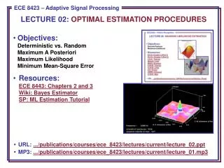
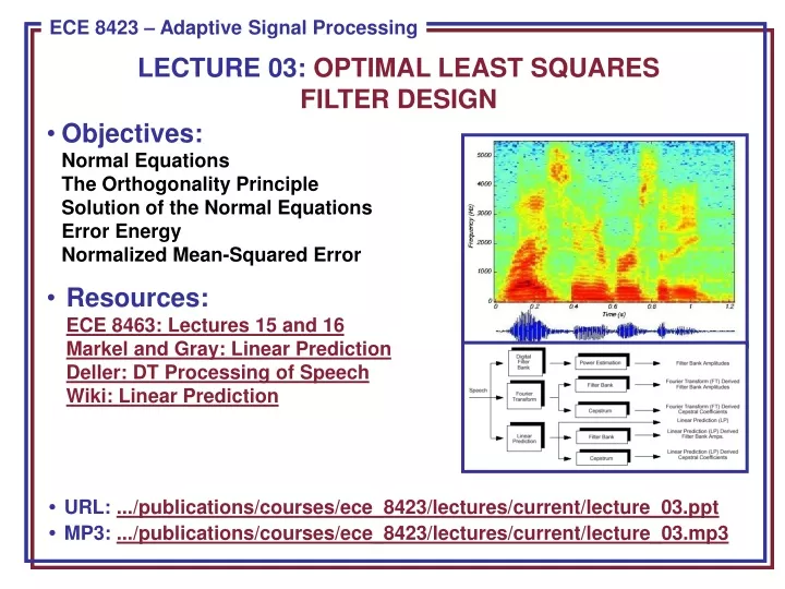
1. LECTURE 03: OPTIMAL LEAST SQUARESFILTER DESIGN • Objectives:Normal EquationsThe Orthogonality PrincipleSolution of the Normal EquationsError EnergyNormalized Mean-Squared Error • Resources:ECE 8463: Lectures 15 and 16Markel and Gray: Linear PredictionDeller: DT Processing of SpeechWiki: Linear Prediction • URL: .../publications/courses/ece_8423/lectures/current/lecture_03.ppt • MP3: .../publications/courses/ece_8423/lectures/current/lecture_03.mp3

2. The Filtering Problem • An input signal, , is filteredusing a linear filter with impulse response, , in such a way that the output, , is as close as possible to some desired signal, . • The performance is measured in terms of the energy of error, . + – • We can define an objective function: • We can write an expression for the error: • We can differentiate with respect toeach coefficient, : • Substituting our expression for the error:

3. The Normal Equations • Combining results: • Equating to zero gives a set of linear algebraic equations known as the normal equations:

4. The Orthogonality Principle • The term normal equations arises from the orthogonality of the input signal and the error, which results from equating the derivatives of J to zero: • It is also common that we “debias”, or remove the DC value, of the input, , such that: • which implies and are uncorrelated. • The error and output are also uncorrelated: • Minimization of a quadratic form produces a single, global, minimum. One way to verify this would be to examine the second derivative. • In addition, the minimization of a quadratic form using a linear filter guarantees linear equations will result. This is attractive because it produces a computationally efficient solution. • We will soon see that such solutions can be derived using basic principles of linear algebra.

5. Autocorrelation and Autocovariance Solutions • For stationary inputs, we can convert the correlation to a traditional autocorrelation: • We can also convert : • The normal equations reduce to: • The solution to this equation is known as the autocorrelation solution. This equation can be written in matrix form using an autocorrelation matrix that is Toeplitz and is very stable. • An alternate form of the solution exists if we use the original normal equation: • This is known as the autocovariance solution because the matrix form of this equation involves a covariance matrix. • We now need to consider the limits on these summations. In a traditional, frame-based approach to signal processing, we have a finite amount of data with which to estimate these functions. In some implementations, data from previous and future frames are used to better estimate these functions at the boundaries of the analysis window.

6. Solutions of the Normal Equations • If we consider the filter to be an infinite length, two-sided (acausal) filter: • We recognize the term on the left as a convolution, and can apply a z-Transform to compute the filter as a ratio of z-Transforms: • If we consider the filter to be of finite length, L: • We can define the filter as a vector of coefficients: • We can define a data vector: • The convolution can be written as a dot product: • The gradient of J can be written as , and .

7. Computation of the Least-Squares Solution • The correlation functions can beestimated in many ways. In typicalapplications, the data is presentedusing a temporal windowingapproach in which weuse an overlapping window. • The most popular method forcomputing the autocorrelationfunction is: • Other common forms are: • Correlation matrices are in general well-behaved (e.g., semi-positive definite), but matrix inversion is computationally costly. Fortunately, highly efficient recursions exist to solve these equations. The covariance matrix can be efficiently inverted using the Cholesky decomposition. The autocorrelation method can be solved recursively using the Levinson recursion.

8. Error Energy • The error energy is a measure of the performance of the filter. • The minimum error is achieved when , which simplifies to: • We can define an error vector: • We can derive an expression for the error in terms of the minimum error: • This shows that the minimum error is achieved by because ,a consequence of the autocorrelation matrix being positive semi-definite. • This also shows that the error energy is a monotonically non-increasing function of L, the length of the filter, because . • This last relation is important because it demonstrates that the accuracy of the model increases as we increase the order of the filter. However, we also risk overfitting the data in the case of noisy data.

9. Normalized Mean-Square Error and Performance • We can define a normalized version of the error by dividing by the variance of the desired signal, : • This bounds the normalized error: • We can define a performance measure in terms of this normalized error: • P is also bounded:

10. Summary • We have introduced the concept of linear prediction in a generalized sense using an adaptive filtering scenario. • We derived equations to estimate the coefficients of the model, and to evaluate the error. • Issue: what happens if our desired signal is white noise? • Next: we will reformulate linear prediction for the specific case of a time series using delayed samples of itself, and view linear prediction as a least-squares digital filter. + –