Long range HETCOR A couple of lectures ago we discussed the HETCOR pulse

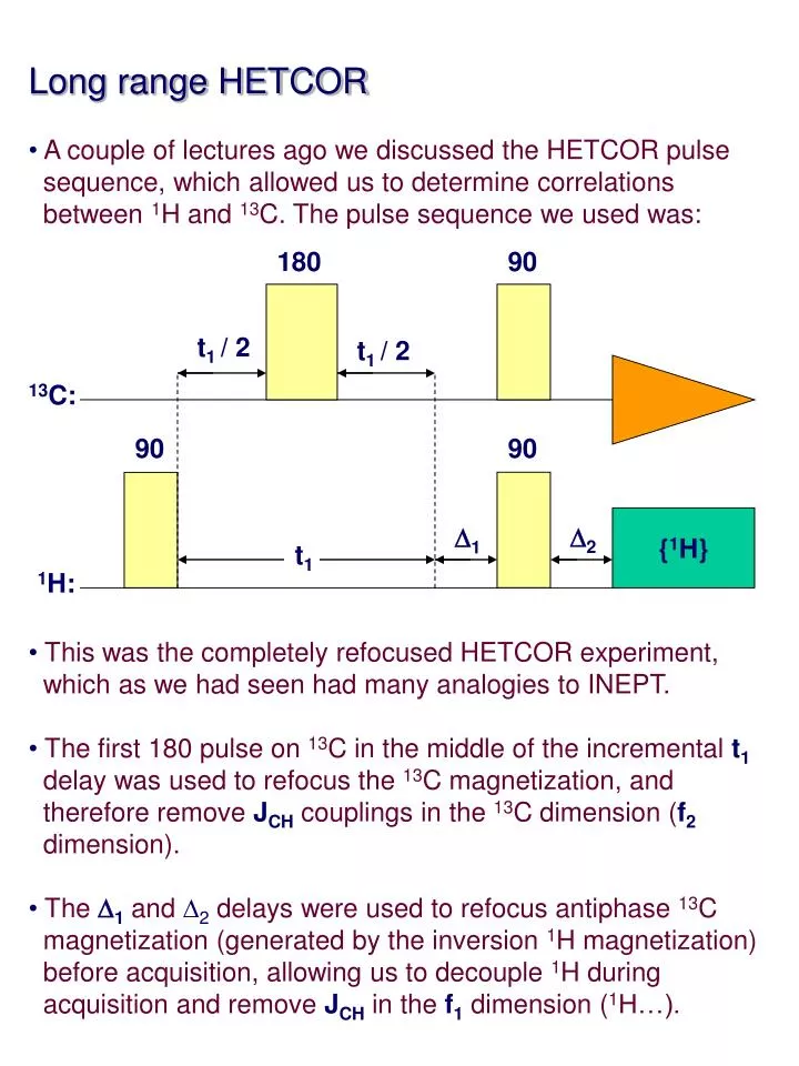
1. Long range HETCOR • A couple of lectures ago we discussed the HETCOR pulse • sequence, which allowed us to determine correlations • between 1H and 13C. The pulse sequence we used was: • This was the completely refocused HETCOR experiment, • which as we had seen had many analogies to INEPT. • The first 180 pulse on 13C in the middle of the incremental t1 • delay was used to refocus the 13C magnetization, and • therefore remove JCH couplings in the 13C dimension (f2 • dimension). • The D1 and D2 delays were used to refocus antiphase 13C • magnetization (generated by the inversion 1H magnetization) • before acquisition, allowing us to decouple 1H during • acquisition and remove JCH in the f1 dimension (1H…). 180 90 t1 / 2 t1 / 2 13C: 90 90 {1H} D1 D2 t1 1H:

2. Long range HETCOR (continued) • The D1 and D2 delays are such that we maximize antiphase • 13C magnetization for 1JCH couplings. That is, D1 and D2 are • in the 2 to 5 ms range (the average 1JCH is ~ 150 Hz, and the • D1 and D2 delays were 1 / 2J). • This is fine to see CH correlations between carbons and • protons which are directly attached (1JCH). Lets see what this • means for camphor, which we discussed briefly in class: • An expansion of the HETCOR spectrum for carbons a and b • would look like: b a f2 (13C) Hb f1 (1H) Ha Hc Ca Cb

3. Long range HETCOR (…) • The problem here is that both carbons a and b are pretty • similar chemically and magnetically: From this data alone we • would not be able to determine which one is which. • It would be nice if we could somehow determine which of the • two carbons is the one closer to the proton at Cc, because • we would unambiguously assign these carbons in camphor: • How can we do this? There is, in principle, a very simple • experiment that relies on long-range CH couplings. • Apart from 1JCH couplings, carbons and protons will show • long-range couplings, which can be across two or three • bonds (either 2JCH or 3JCH). Their values are a lot smaller • than the direct couplings, but are still considerably large, in • the order of 5 to 20 Hz. • Now, how can we twitch the HETCOR pulse sequence to • show us nuclei correlated through long-range couplings? Hb b Ha c a Hc Ca Cb

4. Long range HETCOR (…) • The key is to understand what the different delays in the • pulse sequence do, particularly the D1 and D2 delays. These • were used to refocus antiphase 13C magnetization. For the • 1H part of the sequence: • For the 13C part: • In order to get refocusing, i.e., to get the ‘-3’ and the ‘+5’ • vectors aligned, and in the case of a methine (CH), the D1 • and D2 delays have to be 1 / 2 * 1JCH. So, what would • happen if we set the D1 and D2 delays to 1 / 2 * 2JCH? z y b 90 D1 x x b a y a z y y 5 90 D2 x x x 5 5 3 3 y 3

5. Long range HETCOR (…) • To begin with, D1 and D2 will be in the order of 50 ms instead • of 5 ms, which is much longer than before. What will happen • now is that antiphase 13C magnetization due to 1JCH • couplings will not refocus, and will tend to cancel out. For the • 1H part of the refocusing: • The delay values are now way of the mark for 1JCH, and we • do not have complete inversion of the 1H populations. Now, • for the 13C part: • At the time we decouple 1H, we will almost kill all the 13C • signal that evolved under the effect of 1JCH… z y b a 90 D1 x x b y a z y y < 5 < 5 90 D2 x x x < 3 < 3 y

6. Long range HETCOR (…) • In the end, we’ll se that most of the magnetization that • evolved under the effect of different 1JCHs will be wiped out. • On the other hand, 13C antiphase magnetization that • originated due to 2JCHwill have the right D1 and D2 delays, • so it will behave as we saw before. For 1H: • For 13C: • So in the end, only 13C that have 2JCH couplings will give • rise to correlations in our HETCOR and we will be able to • achieve what we wanted z y b 90 D1 (1 / 2 2JCH) x x b a y a z y y 5 90 x x x 5 5 3 D2 (1 / 2 2JCH) 3 y 3

7. Long range HETCOR (…) • If we take our HETCOR using this values for D1 and D2 , and • if we consider everything working in our favor, we get: • Great. We can now see our long-range 1H-13C coupling, and • we can now determine which CH2 carbon is which in • camphor. Note that we did the whole explanation for CHs for • simplicity, but the picture is pretty much the same for CH2s. • As usual, things never go the way we want.This sequence • has several drawbacks. First, selecting the right D1 and D2 to • see 2JCH over 1JCH is kind of a crap-shot. • Second, we are now talking of pretty long delays D1 and D2 • on top of the variable evolution delay (which is usually in the • order of 10 to 20 ms). We will have a lot of relaxation, not • only of the 13C but of the 1H, during this time, and our signal • will be pretty weak. • Furthermore, since 1H relaxes considerably, the inversion will • vanish away and we don’t get strong correlations. Hb Ha b c Hc a Ca Cb

8. COLOC-HETCOR • How can we avoid these problems? If we want to keep the • idea we have been using, i.e., to refocus 13C magentization • associated with 2JCH, we need to keep the D1 and D2 delays. • Then the only delay that we could, in principle, make shorter • is the variable evolution delay, t1. How do we do this, if we • need this delay to vary from experiment to experiment to get • the second dimension? • The solution is to perform a constant time experiment. This • involves to have an evolution time t1 that is overall constant, • and equal to D1, but have the pulses inside the evolution • progress during this time. The best example of such a pulse • sequence is called COrrelations via LOng-range • Couplings, or COLOC. The pulse sequence is: 180 90 t1 / 2 D2 D1 - t1 / 2 13C: 90 90 180 {1H} t1 / 2 D2 D1 - t1 / 2 1H: D1

9. COLOC-HETCOR (continued) • As you see from the pulse sequence, the D1 period remains • the same, as so does the total t1 period. However, we • achieve the evolution in t1 by shifting the two 180 pulses • through the t1 period constantly from one experiment to the • other. • We can analyze how this pulse sequence works in the same • way we saw how the regular HETCOR works. We’ll see the • analysis for a C-C-H. The first 1H 90 puts 1H magnetization • in the <xy> plane, were it evolves under the effect of JCH • (2JCH in the case of C-C-H) for a period t1 / 2, which is • variable. • The combination of 180 pulses in 1H and 13C inverts the the • 1H magnetization and flips the labels of the 1H vectors: y y 18013C 1801H t1 / 2 ... x x b a a b

10. COLOC-HETCOR (...) • Now, after D1 - t1 / 2, the magnetization continues to • dephase. However, since the total time is D1, we will get the • complete inversion of 1H magnetization, we have the • maximum polarization transfer from 1H to 13C, and we tag • the 13C magnetization with the 1H frequency (which gives us • the correlation…). • Since we always have complete inversion of 1H • magentization and refocusing, we won’t have 2JCH spliting in • the 13C dimension (f1). • Finally, over the D2delay we have refocusing of the 13C • antiphase magnetization, just as in the refocused HETCOR, • and we can decouple protons during acquisition: • The main advantage of this pulse sequence over HETCOR is • that we accomplish the same but in a much shorter time, • because the D1period is included in the t1 evolution. • Furthermore, instead of increasing t1 from experiment to • experiment, we change the relative position of the 180 pulses • to achieve the polarization transfer and frequency labeling. z y y 5 90 D2 x x x 5 5 3 3 y 3