Query Optimization: Relational Queries to Data Mining

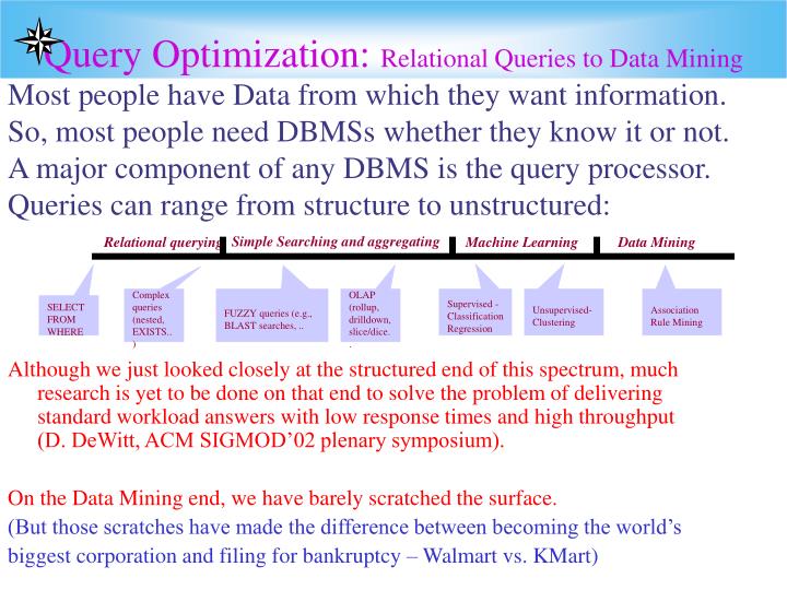
1. Query Optimization: Relational Queries to Data Mining Simple Searching and aggregating Relational querying Machine Learning Data Mining Complex queries (nested, EXISTS..) FUZZY queries (e.g., BLAST searches, .. OLAP (rollup, drilldown, slice/dice.. Supervised - Classification Regression Unsupervised- Clustering Association Rule Mining SELECT FROM WHERE Most people have Data from which they want information. So, most people need DBMSs whether they know it or not. A major component of any DBMS is the query processor. Queries can range from structure to unstructured: Although we just looked closely at the structured end of this spectrum, much research is yet to be done on that end to solve the problem of delivering standard workload answers with low response times and high throughput (D. DeWitt, ACM SIGMOD’02 plenary symposium). On the Data Mining end, we have barely scratched the surface. (But those scratches have made the difference between becoming the world’s biggest corporation and filing for bankruptcy – Walmart vs. KMart)

2. BSM — A Bit Level Decomposition Storage ModelA model of query optimization of all types • Vertical partitioning has been studied within the context of both centralized database system as well as distributed ones. It is a good strategy when small numbers of columns are retrieved by most queries. The decomposition of a relation also permits a number of transactions to execute concurrently. Copeland et al presented an attribute level decomposition storage model (DSM) [CK85] storing each column of a relational table into a separate binary table. The DSM showed great comparability in performance. • Beyond attribute level decomposition, Wong et al further took the advantage of encoding attribute values using a small number of bits to reduce the storage space [WLO+85]. In this paper, we will decompose attributes of relational tables into bit position level, utilize SPJ query optimization strategy on them, store the query results in one relational table, finally data mine using our very good P-tree methods. • Our method offers these advantages: • (1) By vertical partitioning, we only need to read everything we need. This method makes hardware caching work really well and greatly increases the effectiveness of the I/O device. • (2) We encode attribute values into bit vector format, which makes compression easy to do. • (3) SPJ queries can be formulated as Boolean expressions, which facilitates fast implementation on hardware. • (4) Our model is fit not only for query processing but for data mining as well. • [CK85] G.Copeland, S. Khoshafian. A Decomposition Storage Model. Proc. ACM Int. Conf. on Management of Data (SIGMOD’85), pp.268-279, Austin, TX, May 1985. • [WLO+85] H. K. T. Wong, H.-F. Liu, F. Olken, D. Rotem, and L. Wong. Bit Transposed Files. • Proc. Int. Conf. on Very Large Data Bases (VLDB’85), pp.448-457, Stockholm, Sweden, 1985.

3. SPJ Query Optimization Strategies - One-table Selections • There are two categories of queries in one-table selections: Equality Queries and Range Queries. Most techniques [WLO+85, OQ97, CI98] used to optimize them employ encoding schemes – equality encoding and range encoding. Chan and Ioannidis [CI99] defined a more general query format called interval query. An interval query on attribute A is a query of the form “x≤A≤y” or “NOT (x≤A≤y)”. It can be an equality query or a range query when x or y satisfies different kinds of conditions. • We defined interval P-trees in previous work [DKR+02], which is equivalent to the bit vectors of corresponding intervals. So for each restriction in the form above, we have one corresponding interval P-tree. The ANDing result of all the corresponding interval P-trees represents all the rows satisfy the conjunction of all the restriction in the where clause. • [CI98] C.Y. Chan and Y. Ioannidis. Bitmap Index Design and Evaluation. Proc. ACM Intl. Conf. on Management of Data (SIGMOD’98), pp.355-366, Seattle, WA, June 1998. • [CI99] C.Y. Chan and Y.E. Ioannidis. An Efficient Bitmap Encoding Scheme for Selection Queries. Proc. ACM Intl. Conf. on Management of Data (SIGMOD’99), pp.216-226, Philadephia, PA, 1999. • [DKR+02] Q. Ding, M. Khan, A. Roy, and W. Perrizo. The P-tree algebra. Proc. ACM Symposium Applied Computing (SAC 2002), pp.426-431, Madrid, Spain, 2002. • [OQ97] P. O’Neill and D. Quass. Improved Query Performance with Variant Indexes. Proc. ACM Int. Conf. on Management of Data (SIGMOD’97), pp.38-49, Tucson, AZ, May 1997.

4. Vertical Select-Project-Join (SPJ) Queries A Select-Project-Join query has joins, selections and projections. Typically there is a central fact relation to which several dimension relations are to be joined (standard STAR DW) E.g., Student(S), Course(C), Enrol(E) STAR DB below (bit encoding is shown in reduced font italics for certain attributes) S|s____|name_|gen|C|c____|name|st|term| E|s____|c____|grade | |0 000|CLAY |M 0||0 000|BI |ND|F 0| |0 000|1 001|B 10| |1 001|THAIS|M 0||1 001|DB |ND|S 1| |0 000|0 000|A 11| |2 010|GOOD |F 1||2 010|DM |NJ|S 1| |3 011|1 001|A 11| |3 011|BAID |F 1||3 011|DS |ND|F 0| |3 011|3 011|D 00| |4 100|PERRY|M 0||4 100|SE |NJ|S 1| |1 001|3 011|D 00| |5 101|JOAN |F 1||5 101|AI |ND|F 0| |1 001|0 000|B 10| |2 010|2 010|B 10| |2 010|3 011|A 11| |4 100|4 100|B 10| |5 101|5 101|B 10| Vertical bit sliced (uncompressed) attrs stored as: S.s2S.s1S.s0S.gC.c2C.c1C.c0C.tE.s2E.s1E.s0E.c2E.c1E.c0E.g1 E.g0 0 0 0 0 0 0 0 00 0 0 0 0 1 1 0 0 0 1 0 0 0 1 10 0 0 0 0 0 1 1 1 0 0 0 1 0 0 10 0 1 0 1 1 0 0 1 0 1 1 1 0 1 00 0 1 0 0 0 1 0 0 1 0 1 0 1 0 10 1 1 0 1 1 1 1 0 1 1 1 0 1 1 00 1 1 0 1 1 0 0 0 1 0 0 1 0 1 0 0 1 0 0 0 1 1 1 1 0 0 1 0 0 1 0 1 0 1 1 0 1 1 0 Vertical (un-bit-sliced) attributes are stored:S.name C.nameC.st |CLAY ||BI | |ND| |THAIS||DB | |ND| |GOOD ||DM | |NJ| |BAID ||DS | |ND| |PERRY||SE | |NJ| |JOAN ||AI | |ND|

5. When ≥ 1 join is required and there are >1 join attributes (i.e., bushy query tree): e.g., the following bushy SPJ on Student, Course, Offerings, Rooms, Enrollments files: O.o2 0 0 0 0 1 1 1 1 R:r cap |0 00|30 11| |1 01|20 10| |2 10|30 11| |3 11|10 01| SELECTS.n, C.nFROMS, C, O, R, E WHERES.s=E.s&C.c=O.c&O.o=E.o&O.r=R.r &S.g=M&C.r=2&E.g=A&R.c=20; S:s ngen |0 000|A|M| |1 001|T|M| |2 010|S|F| |3 011|B|F| |4 100|C|M| |5 101|J|F| R.r1 0 0 1 1 R.r0 0 1 0 1 R.c1 1 1 1 0 R.c0 1 0 1 1 O :o c r |0 000|0 00|0 01| |1 001|0 00|1 01| |2 010|1 01|0 00| |3 011|1 01|1 01| |4 100|2 10|0 00| |5 101|2 10|2 10| |6 110|2 10|3 11| |7 111|3 11|2 10| E:s o grade |0 000|1 001|2 10| |0 000|0 000|3 11| |3 011|1 001|3 11| |3 011|3 011|0 00| |1 001|3 011|0 00| |1 001|0 000|2 10| |2 010|2 010|2 10| |2 010|7 111|3 11| |4 100|4 100|2 10| |5 101|5 101|2 10| S.s2 0 0 1 1 0 0 S.s1 0 0 0 0 1 1 S.s0 0 1 0 1 0 1 S.n A T S B C J S.g M M F F M F O.o1 0 0 1 1 0 0 1 1 O.o0 0 1 0 1 0 1 0 1 O.c1 0 0 0 0 1 1 1 1 O.c0 0 0 1 1 0 0 0 1 O.r1 0 0 0 0 0 1 1 1 O.r0 1 1 0 1 0 0 1 0 E.s2 0 0 0 0 0 0 0 0 1 1 E.s1 0 0 1 1 0 0 1 1 0 0 E.s0 0 0 1 1 1 1 0 0 0 1 E.o2 0 0 0 0 0 0 0 1 1 1 E.o1 0 0 0 1 1 0 1 1 0 0 E.o0 1 0 1 1 1 0 0 1 0 1 E.g1 1 1 1 0 0 1 1 1 1 1 E.g0 0 1 1 0 0 0 0 1 0 0 C:c ncred |0 00|B|1 01| |1 01|D|3 11| |2 10|M|3 11| |3 11|S|2 10| C.c1 0 0 1 1 C.n B D M S C.c0 0 1 0 1 C.r1 0 1 1 1 C.r0 1 1 1 0

6. S.s2 0 0 1 1 0 0 S.s1 0 0 0 0 1 1 S.s0 0 1 0 1 0 1 S.n A T S B C J SM 1 1 0 0 1 0 S.g M M F F M F O.o2 0 0 0 0 1 1 1 1 O.o1 0 0 1 1 0 0 1 1 O.o0 0 1 0 1 0 1 0 1 O.c1 0 0 0 0 1 1 1 1 O.c0 0 0 1 1 0 0 0 1 O.r1 0 0 0 0 0 1 1 1 O.r0 1 1 0 1 0 0 1 0 R.r1 0 0 1 1 R.r0 0 1 0 1 R.c1 1 1 1 0 R.c1 1 1 1 0 R.c0 1 0 1 1 R.c’0 0 1 0 0 E.s2 0 0 0 0 0 0 0 0 1 1 E.s1 0 0 1 1 0 0 1 1 0 0 E.s0 0 0 1 1 1 1 0 0 0 1 E.o2 0 0 0 0 0 0 1 0 1 1 E.o1 0 0 0 1 1 0 1 1 0 0 E.o0 1 0 1 1 1 0 0 1 0 1 E.g1 1 1 1 0 0 1 1 1 1 1 E.g1 1 1 1 0 0 1 1 1 1 1 E.g0 0 1 1 0 0 0 0 1 0 0 E.g0 0 1 1 0 0 0 0 1 0 0 For selections, S.g=MC.r=2E.g=AR.c=20 create selection masks (note that C.r=2 is coded in binary as 10b EgA 0 1 1 0 0 0 0 1 0 0 C.c1 0 0 1 1 C.n B D M S C.c1 0 1 0 1 C.r1 0 1 1 1 C.r1 0 1 1 1 C.r2 1 1 1 0 C.r’2 0 0 0 1 Rc20 0 1 0 0 Cr2 0 0 0 1 Apply selection masks (Zero out numeric values, blanked out others). S.s2 0 0 0 0 0 0 S.s1 0 0 0 0 1 0 S.s0 0 1 0 0 0 0 S.n A T C O.o2 0 0 0 0 1 1 1 1 O.o1 0 0 1 1 0 0 1 1 0 0 1 0 1 0 1 0 1 O.c1 0 0 0 0 1 1 1 1 O.c0 0 0 1 1 0 0 0 1 O.r1 0 0 0 0 0 1 1 1 O.r0 1 1 0 1 0 0 1 0 R.r1 0 0 0 0 R.r0 0 1 0 0 E.s2 0 0 0 0 0 0 0 0 0 0 E.s1 0 0 1 0 0 0 0 1 0 0 E.s0 0 0 1 0 0 0 0 0 0 0 E.o2 0 0 0 0 0 0 0 1 0 0 E.o1 0 0 0 0 0 0 0 1 0 0 E.o0 0 0 1 0 0 0 0 1 0 0 C.c1 0 0 0 1 C.n S C.c0 0 0 0 1 SELECTS.n, C.nFROMS, C, O, R, E WHERES.s=E.s&C.c=O.c&O.o=E.o&O.r=R.r &S.g=M&C.r=2&E.g=A&R.c=20;

7. S.s2 0 0 0 0 0 0 S.s1 0 0 0 0 1 0 S.s0 0 1 0 0 0 0 S.n A T C O.o2 0 0 0 0 1 1 1 1 O.o1 0 0 1 1 0 0 1 1 O.o0 0 1 0 1 0 1 0 1 O.c1 0 0 0 0 1 1 1 1 O.c0 0 0 1 1 0 0 0 1 O.r1 0 0 0 0 0 1 1 1 O.r1 0 0 0 0 0 1 1 1 O.r0 1 1 0 1 0 0 1 0 O’.r0 0 0 1 0 1 1 0 1 R.r1 0 0 0 0 R.r0 0 1 0 0 Rc20 0 1 0 0 E.s2 0 0 0 0 0 0 0 0 0 0 E.s1 0 0 1 0 0 0 0 1 0 0 E.s0 0 0 1 0 0 0 0 0 0 0 E.o2 0 0 0 0 0 0 0 1 0 0 E.o1 0 0 0 0 0 0 0 1 0 0 E.o0 0 0 1 0 0 0 0 1 0 0 For the joins, S.s=E.sC.c=O.cO.o=E.oO.r=R.r,one approach is to follow an indexed nested loop like method (note that the P-trees themselves are self indexing). C.c1 0 0 0 1 C.n S C.c0 0 0 0 1 The join O.r=R.ris simply part of a selection on O (R doesn’t contribute output nor participate in any further operations) Use the Rc20-masked R as the inner relation and O as the r-indexed outer relation) to produce a further selection mask for O. Get 1st R.r value, 01b Mask the corresponding O tuples, PO.r1^P’O.r0 OM 0 0 0 0 0 1 0 1 O.o2 0 0 0 0 0 1 0 1 O.o1 0 0 0 0 0 0 0 1 O.o0 0 0 0 0 0 1 0 1 O.c1 0 0 0 0 0 1 0 1 O.c0 0 0 0 0 0 0 0 1 This is the only R.r value (if there were more, one would do the same for each, then OR those masks to get the final O-mask). Next, we apply the O-mask, OM to O SELECTS.n, C.nFROMS, C, O, R, E WHERES.s=E.s&C.c=O.c&O.o=E.o&O.r=R.r &S.g=M&C.r=2&E.g=A&R.c=20;

8. O.o2 0 0 0 0 0 1 0 1 O.o1 0 0 0 0 0 0 0 1 O.o0 0 0 0 0 0 1 0 1 O.c1 0 0 0 0 0 1 0 1 O.c1 0 0 0 0 0 1 0 1 O.c0 0 0 0 0 0 0 0 1 O.c0 0 0 0 0 0 0 0 1 E.s2 0 0 0 0 0 0 0 0 0 0 E.s1 0 0 1 0 0 0 0 1 0 0 E.s0 0 0 1 0 0 0 0 0 0 0 E.o2 0 0 0 0 0 0 0 1 0 0 E.o2 0 0 0 0 0 0 0 1 0 0 E.o1 0 0 0 0 0 0 0 1 0 0 E.o1 0 0 0 0 0 0 0 1 0 0 E.o0 0 0 1 0 0 0 0 1 0 0 E.o0 0 0 1 0 0 0 0 1 0 0 S’.s2 1 1 0 0 1 0 S.s2 0 0 0 0 0 0 S.s1 0 0 0 0 1 0 S.s1 0 0 0 0 1 0 S’.s0 1 0 0 0 1 0 S.s0 0 1 0 0 0 0 S.n A T C C.c1 0 0 0 1 C.c0 0 0 0 1 C.n S For the final 3 joins C.c=O.cO.o=E.o E.s=S.sthe same indexed nested loop like method can be used. OM 0 0 0 0 0 0 0 1 EM 0 0 0 0 0 0 0 1 0 0 Get 1st masked C.c value, 11b Mask corresponding O tuples: PO.c1^PO.c0 Get 1st masked O.o value, 111b Mask corresponding E tuples: PE.o2^PE.o1^PE.o0 SM 0 0 0 0 1 0 Get 1st masked E.s value, 010b Mask corresponding S tuples: P’S.s2^PS.s1^P’S.s0 Get S.n-value(s), C, pair it with C.n-value(s), S, output concatenation, C.nS.n S C There was just one masked tuple at each stage in this example. In general, one would loop through the masked portion of the extant domain at each level (thus,Indexed Horizontal Nested Loop or IHNL) SELECTS.n, C.nFROMS, C, O, R, E WHERES.s=E.s&C.c=O.c&O.o=E.o&O.r=R.r &S.g=M&C.r=2&E.g=A&R.c=20;

9. O.o1 0 0 0 0 0 1 0 1 O.o2 0 0 0 0 0 0 0 1 O.o3 0 0 0 0 0 1 0 1 O.c1 0 0 0 0 0 1 0 1 O.c2 0 0 0 0 0 0 0 1 E.s1 0 0 0 0 0 0 0 0 0 0 E.s2 0 0 1 0 0 0 0 1 0 0 E.s3 0 0 1 0 0 0 0 0 0 0 E.o1 0 0 0 0 0 0 0 1 0 0 E.o2 0 0 0 0 0 0 0 1 0 0 E.o3 0 0 1 0 0 0 0 1 0 0 S.s1 0 0 0 0 0 0 S.s2 0 0 0 0 1 0 S.s3 0 1 0 0 0 0 S.n A T C C.c1 0 0 0 1 C.n S C.c1 0 0 0 1 Having done the query tree sequentially (selections first, then joins and projections) it occurs to me that the entire query tree could be done in one combined step by looping through the masked C tuples, for each C.n value, determine if there is an S.n value that should be paired with it by logical operations output those S.n, C.n pair(s), if any, else go to the next masked C.n value. Does this lead to a one-pass vertical query optimizer?!?!?! Can the indexed nested loop like algorithm be modified to loop horizontally? (across bit positions, rather than down tuples?) SELECTS.n, C.nFROMS, C, O, R, E WHERES.s=E.s&C.c=O.c&O.o=E.o&O.r=R.r &S.g=M&C.r=2&E.g=A&R.c=20;

10. DISTINCT Keyword, GROUP BY Clause, ORDER BY Clause, HAVING Clause and Aggregate Operations • Duplicate elimination after a projection (SQL DISTINCT keyword) is one of the most expensive operations in query optimisation. In general, it is as expensive as the join operation. However, in our approach, it can automatically be done while forming the output tuples (since that is done in an order). While forming all output records for a particular value of the ORDER BY attribute, duplicates can be easily eliminated without the need for an expensive algorithm. • The ORDER BY and GROUP BY clauses are very commonly used in queries and can require a sorting of the output relation. However, in our approach, if the central relation is chosen to be the one with the sort attribute and the surrogation is according to the attribute order (typically the case – always the case for numeric attributes), then the final output records can be put together and aggregated in the requested order without a separate sort step at no additional cost. Aggregation operators such as COUNT, SUM, AVG, MAX, and MIN can be implemented without additional cost during the output formation step and any HAVING decision can be made as output records are being composed, as well (See Yue Cui’s Master’s thesis in NDSU library for vertical aggregation computations using P-trees.) • If the Count aggregate is requested by itself, we note that P-trees automatically provide the full counts for any predicate with just one multiway AND operation.

11. Combining Data Mining and Query Processing • Many data mining request involve pre-selection, pre-join, and pre-projection on a database to isolate the specific data subset to which the data mining algorithm is to be applied. For example, in the above database, one might be interested in all Association Rules of a given support threshold and confidence threshold but only on the result relations of the complex SPJ query shown. The brute force way to do this is to first join all relations into one universal relation and then to mine that gigantic relation. This is not a feasible solution in most cases due to the size of the resulting universal relation. Furthermore, often some selection on that universal relation is desirable prior to the mining step. • Our approach accommodates combinations of querying and data mining without necessitation the creation of a massive universal relation as an intermediate step. Essentially, the full vertical partitioning and P-trees provide a selection and join path which can be combined with the data mining algorithm to produce the desired solution without extensive processing and massive space requirements. The collection of P-trees and BSQ files constitute a lossless, compressed version of the universal relation. Therefore the above techniques, when combined with the required data mining algorithm can produce the combination result very efficiently and directly.

12. E:s o grade |0 000|1 001|2 10| |0 000|0 000|3 11| |3 011|1 001|3 11| |3 011|3 011|0 00| |1 001|3 011|0 00| |1 001|0 000|2 10| |2 010|2 010|2 10| |2 010|7 111|3 11| |4 100|4 100|2 10| |5 101|5 101|2 10| O :o c r |0 000|0 00|0 01| |1 001|0 00|1 01| |2 010|1 01|0 00| |3 011|1 01|1 01| |4 100|2 10|0 00| |5 101|2 10|2 10| |6 110|2 10|3 11| |7 111|3 11|2 10| S:s ngen |0 000|A|M| |1 001|T|M| |2 010|S|F| |3 011|B|F| |4 100|C|M| |5 101|J|F| C:c ncred |0 00|B|1 01| |1 01|D|3 11| |2 10|M|3 11| |3 11|S|2 10| R:r cap |0 00|30 11| |1 01|20 10| |2 10|20 10| |3 11|10 01| C.c1 0 0 1 1 R.r1 0 0 1 1 R.r0 0 1 0 1 R.c1 1 1 1 0 R.c0 1 0 0 1 C.c0 0 1 0 1 C.n B D M S C.r1 0 1 1 1 C.r0 1 1 1 0 O.o2 0 0 0 0 1 1 1 1 O.o1 0 0 1 1 0 0 1 1 O.o0 0 1 0 1 0 1 0 1 O.c1 0 0 0 0 1 1 1 1 O.c0 0 0 1 1 0 0 0 1 O.r1 0 0 0 0 0 1 1 1 O.r0 1 1 0 1 0 0 1 0 S.s2 0 0 1 1 0 0 S.s1 0 0 0 0 1 1 S.s0 0 1 0 1 0 1 S.n A T S B C J S.g 0 0 1 1 0 1 E.s2 0 0 0 0 0 0 0 0 1 1 E.s1 0 0 1 1 0 0 1 1 0 0 E.s0 0 0 1 1 1 1 0 0 0 1 E.o2 0 0 0 0 0 0 0 1 1 1 E.o1 0 0 0 1 1 0 1 1 0 0 E.o0 1 0 1 1 1 0 0 1 0 1 E.g1 1 1 1 0 0 1 1 1 1 1 E.g0 0 1 1 0 0 0 0 1 0 0 Horizontal Indexed Nested Loop Join??? SELECT*FROMS,EWHERES.s=E.s 1st if 0<rc(S.s2) thenif rc(S.s2)<|S| thenif 0<rc(S.s1)^ thenif rc(S.s1)<|S| thenif 0<rc(S.s0) thenif rc(S.s0)<|S| then… So depth-first traversal down the bitslice tree for S.s, skipping all values that are not present, and for each S.s value that is present, one and gives that value P-tree in E (index into E) so optimal retrieval can be done. If the Ptrees are organized according to physical boundaries as below, then is there a P-tree based Hybrid Hash join that allows us to avoid excessive rereads of extents? It seems clear that compressing bit vectors into P-trees based, not on 1/2d boundaries, but on page and extent boundaries is important. Use the Dr. Md Masum Serazi approach, but with the following levels (possibly collapsing levels 0 and 1 together) The level-0 fanout is the bfr of the page blocks. The level-1 fanout is the extent size (# of blocks per extent). The level-2 fanout is the (maximum) number of extents per file. The level-3 fanout is the number of files in the DB The real advantage of this approach may to apply it to join algorithms where the location of join Attribute values is known ( see V. Goli’s thesis) since we know the location of all values Through ANDs.

13. Graph G=(N,E) is (T,I)-bipartite iff N=T!I and e={e1,e2}E, if e1T [I] then e2I [T]. WOLOG write e={eT,eI} (E is directed from T to I e=(eT,eI) ) E={ {ek,T,ek,I} | k=1..|E|} or the edge relationship can be expressed as E.s2 1 0 0 0 0 0 0 0 1 1 0 0 0 0 1 1 0 0 0 0 0 0 1 E.s1 0 0 1 1 0 0 1 1 0 0 0 0 0 0 0 0 1 1 1 0 0 0 0 E.s0 0 0 0 1 1 0 1 1 0 0 0 0 0 0 0 0 0 0 0 1 0 0 0 E.g 0 0 0 1 1 0 1 1 0 0 0 0 0 0 0 0 0 0 0 1 0 0 0 E.c1 0 0 0 1 0 0 0 1 0 0 0 0 0 0 0 0 0 1 1 0 0 1 0 E.c0 1 0 0 0 1 0 1 1 0 1 0 0 0 0 0 0 0 1 0 1 1 0 0 tIset, ET= { (t,Iset(t) | tT and Iset(t)={i|{t,i}E} iTset, EI= { (i,Iset(i) | where Iset(i)={t | {t,i}E} tImap, ETb={ (t,b1,...,b|I|) | where bk=1 iff ek,T=t} iTmap, EIb={ (i,b1,...,b|T|) | where bk=1 iff ek,I=t} Given a star schema with fact, E and dimensions, S, C. E is a ER-relationship between entities, S and C and is therefore a bipartite graph, G=(N,E) where N is the disjoint union of S and C. Given a join S.s with E.s, JoinIndex (JI) is a relationship between S and E, giving a bipartite graph, G=(S!E,JI). The sEmap of this relationship is the association matrix of Qiang Ding's thesis. S.s2 0 0 0 0 1 1 1 1 S.s1 0 0 1 1 0 0 1 1 S.s0 0 1 0 1 0 1 0 1 S.a 1 1 0 0 1 0 0 0 C.c1 0 0 1 1 C.c0 0 1 0 1 C.n 1 0 0 1