Download
1 / 23
230 likes | 395 Views
Segmenting the human genome using large-scale RNAi perturbations. Gregoire Pau , Oleg Sklyar, Wolfgang Huber EMBL-EBI Cambridge Florian Fuchs, Christoph Budjan, Thomas Horn, Michael Boutros DKFZ Heidelberg. Experimental setup. Human HeLa cells Genome-wide RNAi knockdowns (22839 genes)

E N D
Segmenting the human genome using large-scale RNAi perturbations Gregoire Pau, Oleg Sklyar, Wolfgang Huber EMBL-EBI Cambridge Florian Fuchs, Christoph Budjan, Thomas Horn, Michael Boutros DKFZ Heidelberg
Experimental setup • Human HeLa cells • Genome-wide RNAi knockdowns (22839 genes) • Incubation for 48h • Staining using DNA (DAPI), Tubulin (Alexa), Actin (TRITC) • Readout: color microscopy images CD3EAP
Microscopy images readout wt- wt- wt- BTDBD3 CEP164 CD3EAP
Motivation • Biological questions • What are the most striking phenotypes ? • What are the gene KDs that give rise to the same phenotypes ? • Can we infer a gene function from its phenotype ? • Computational point of view • Definition of the gene phenotypic profile • Definition of a phenotypic distance
Gene phenotypic profile • Quantitative phenotypic profile expressed by a population of cells • Not a cell phenotype ! • Gene phenotypic profile: • Number of cells • Median cell features (size, eccentricity, …) • Cell types distribution (normal, mitotic, condensed, protruded…) CEP164 CD3EAP
Gene phenotypic profile computation • Done by imageHTS • Bioconductor R package • Works for our screen, generalization needs to be worked out • Open-source free software • To be released • Rely on EBImage • Bioconductor R package • Low-level basic image processing (IO, matrix algebra, filtering, morphological operators…) • Available open-source free software
Computational workflow Image Segmentation Cells Features extraction Cells features CEP164 Classification Intensity = 1778 Cell size = 421 Eccentricity = 1.08 Actin.intensity = 124 Tubulin.intensity = 94 DNA.intensity = 74 Nucleus.size = 46 Actin.hz11 = 17.4 Actin.hz12 = 11.3 Tubulin.hz11 = 8.4 Nucleus.hz11 = 3.4 ... Cell types Metaphase Phenoprinting Gene phenotype
Segmentation • Isolating cells from an image • Using a prior cell model • Iterative adaptative thresholding + Voronoi tesselation Cells are 2D connected sets. Cell boundaries are delimited by a Tubulin cytoskeleton and maybe some actin protusions. Cells contains at least one nucleus. Cell size is bounded. A nucleus cannot be bigger than the cell and has a bounded size. Z = A + T Nmask = (H - Hm) > t1 Cmask = (Zn > t2) t2 must fulfill (Tn > v) Cmask & (An >v) Cmask …
Segmentation • Results: • Accurate results if cells are not too packed • Superposition is hard to handle
Cell features • Quantitative characterization of a cell morphology • 51 selected features: • Geometric (intensity, size, perimeter, eccentricity…) • Texture (Haralick, Zernike moments…) on each channel • Miscellaneous features (joint channel texture, …)
Cell classification • Cells are classified according to their numerical features • Supervised learning using SVM • Using 8 classes and a training set of ~3000 cells: Actin Fiber Lamellipodia Big cells Metaphase Condensed Normal Debris Protusion
Cell classification • Results: • Classification performance (5-fold CV) on TS: ~85 %
Gene phenotypic profile • Quantitative descriptor of a gene phenotype: • Using 13 phenotypic traits CEP164 n int siz ecc Nint Nsiz NCsiz AF BC M LA P Z 128 1054.74 25.56 0.6491 12.752 373.28 0.237 2 7 15 0 17 2 CEP164
Gene phenoprint & phenotypic distance • Goal: • Cut off the variability of the phenotypic traits • Keep only the significant trends • For each phenotypic trait: • Use of a parametric sigmoid transform • Blue: significant decrease: [-1,-0.5] • Boring zone: [-0.5,0.5] • Red: significant increase: [0.5,1] • 20 parameters (, )k are to be determined • Phenotypic distance defined as the L1 distance between 2 phenoprints
Distance learning • Ideas: • Knockdowns of interacting gene pairs lead more likely to similar phenotypes than random gene pairs • Distances of gene pairs picked on STRING should be lower ingeneral than random gene pairs • Distance learning: • Let D+ the set of all pairwise gene distances picked on STRING • Let D- the set of all pairwise gene distances picked randomly • Goal: find the parameters k and k that best separate D+ and D-
Gene phenoprints • Results: • Among the 22839 gene KDs,1891 show non-null phenoprints • Computation time: ~12 hours on a cluster of 30 CPUs
Extreme phenotypes • Most distant phenoprints from the negative controls • Binucleated • Large cells phenotype ADRB2 KIAA0363
Extreme phenotypes • Condensed phenotype • Elongated STK39 STK39 TENC1 LOC51693 KCNT1 LOC51693 KCNT1
Phenotypic map Elongated phenotypes
Phenotypic map Mitotic phenotypes
Secondary assays • Gene function inference • Some genes are well-known to be involved in DNA repair • CLSPN, RRM1… were showing interesting phenoprints ! • Genes showing similar phenoprints are good candidates for retest • Selection: • Among the 1891 non-null phenoprints • 693 genes were selected for retest • 284 genes shown reproducible phenotypes on U2OS cells • Secondary assays • To assess the implication of genes in DNA repair processes • Genotoxic assays, direct foci detection • Ongoing experiments…
Conclusion • Fully automated phenotyping method from microscopy images • Efficient approach to associate new genes to known functional modules