Download
1 / 16
160 likes | 280 Views
Reliability-Based Timepoint Schedules for Long Headway Transit Routes. Peter G. Furth, Northeastern University with Theo H.J. Muller, Delft University of Technology. Outline. Translating Reliability into User Cost Operations model Segment running time Timepoint holding

E N D
Reliability-Based Timepoint Schedules for Long Headway Transit Routes Peter G. Furth, Northeastern University with Theo H.J. Muller, Delft University of Technology
Outline • Translating Reliability into User Cost • Operations model • Segment running time • Timepoint holding • Layover and dispatch holding • Example results
Reliability Affects Passenger Travel Time • Passengers arrive so that P[miss the bus] < 2% • Passengers budget for 95-percentile [wait + ride] time • Potential Travel Time = Budgeted Travel Time – mean [Wait + Ride Time]
Passenger Travel Cost Components Waiting Time: $9/hr Riding Time: $6/hr Potential Travel Time: $4.5/hr Reliability has been captured: Cost = f(Tails of departure and arrival time distributions) Note: Estimating tails requires archived AVL data.
Operating Cost for a Route with Holding = Cycle Time cSchedule = Design Parameter • Can be fixed or optimized cactual = an outcome, the sum of 3 components: • Mean uncontrolled running time • Mean holding time (running time supplement) • Mean layover time (layover slack) Inconsistent unless cactual ≈ cSchedule • Steady state: f(StartDeviationcycle n) ≈f(StartDeviationcycle n+1)
Operations Model Segments (includes necessary dwell time) • Random, independent running times • Ideally, get distribution from AVL data Timepoints • Hold early arrivals • Add random holding supplement End of Line • Add a random needed layover to become “Ready” • Hold early “Ready” • Add random dispatch supplement
Timepoints: Random Holding Supplement Holding Supplement (min)
1 6 End of Line: Needed Layover and Dispatch Supplement Needed Layover (min) Dispatch Supplement (min)
Layover Model: Planning ViewLabor policies on minimum layover constrain cSchedule Finding: • Unreliable service: reliability governs optimal cSchedule • Highly reliable service: labor policy governs
Analysis • Track discretized probability distributions using MatLab • 2 Warm-up cycles to achieve quasi-steady state • Example route • 17 stops, 16 segments • mean running time = 40 min, s = 5 min for base case • mean boardings = 74, max load = 36 pax • Optimize w.r.t. two overlapping schedule parameters • Cycle supplement = CycleTime – MeanUncontrolledRunningTime • Running Time supplement = ScheduledRunningTime – MeanUncontrolledRunningTime
$40 riding time $20 operating cost $0 -15.0 -10.0 -5.0 0.0 5.0 10.0 15.0 potential travel time -$20 total cost -$40 waiting time -$60 Running Time Supplement (min) Cost vs. Running Time SupplementOptimized cycle length
0.40 0.30 Total holding 0.20 Layover holding 0.10 Timepoint holding -15.0 -10.0 -5.0 0.0 5.0 10.0 15.0 Running Time Supplement (min) Slack Distributions vs. Running Time Supplement cScheduleoptimized; dashed line = only 1 timepoint
σroute = 3 min σroute = 5 σroute = 7 (Bars) Change in Cost (Base = No Timepoints) ($/trip) $0 3.5 (Lines) Schedule Supplement as multiple of σroute Cycle suppl, σroute=3 -$10 3 Cycle suppl, σroute=5 -$20 2.5 Cycle suppl, σroute=7 -$30 2 RT suppl, σroute=7 -$40 1.5 RT suppl, σroute=5 -$50 1 RT suppl, σroute=3 -$60 0.5 -$70 0 0 1 3 7 14 Numberof Timepoints Cost vs. Number of Timepoints
3.00 Cycle time supplement 2.00 1.00 Running time supplement 0.00 2.0 3.0 4.0 5.0 6.0 7.0 8.0 s (min) route Optimal Schedule Supplements vs sroutedashed line for a single timepoint
Conclusion and Remarks • Archived AVL data makes reliability analysis possible • Capturing reliability in the cost function facilitates tradeoff against riding time and operating cost; contrast rules of thumb • Schedules should probably have more en-route slack • To a large degree, en-route slack and recovery slack simply substitute for one another, meaning en-route slack can be added without increasing cycle time • Amount of en-route & layover slack are not easily calculated • Optimal departure time depends on boardings & other factors • On more reliable routes, layover is governed by operator rest needs • What about operator behavior? • What about short headway service? • What about passengers who make transfers?