Download
1 / 51
510 likes | 691 Views
Uncertainty Quantification with Experimental Data and Complex System Models. Trent Russi Ph.D. Seminar Spring 2010. Pathway diagram for methane combustion [Turns]. Methane Combustion: CH 4 + 2O 2 CO 2 + 2H 2 O. Model of natural gas chemical kinetics

E N D
Uncertainty Quantification with Experimental Data and Complex System Models Trent Russi Ph.D. Seminar Spring 2010
Pathway diagram for methane combustion [Turns] Methane Combustion: CH4 + 2O2 CO2 + 2H2O • Model of natural gas chemical kinetics • Purpose: Used to predict heat release and concentrations over a wide scale, from work production to pollutant formation. • A current model includes 53 chemical species, 325 reactions (with unknown rates)
E3 Experiment1 Experiment2 Experimental data • Example Experiment Attributes: • Shock-tube Ignition Delay • Maximum CH3 concentration in Shocktube • Laminar Flame Speed • … Experimentally derived value (attribute) ExperimentUncertainty Uncertain Reaction parameters Experiment attribute model • What do experiments tell us about the reaction parameters? • Can this information be used to predict the outcome of future experiments?
A Toy Example Prior Knowledge Bounds on valid domain of Bounds on valid domain of
A Toy Example Reported Domain
A Toy Example Reported Domain
A Toy Example Feasible Set of Parameters Reported ranges don’t intersect! Looks like an inconsistency.
Dataset Prior-knowledge “Hypercube”, Constraints imposed by models and experimental data: All constraints combine to form a “Feasible Set” of parameter values:
Consistency • A dataset is called consistent if the Feasible set is nonempty:i.e. there exist a parameter vector that satisfies all prior information parameter constraints and experiment constraints
Consistency Measure • How much can the uncertainty decrease such that the dataset is consistent? • Off-the-shelf nonlinear optimization solvers (e.g. fmincon) provide a lower bound • implies consistency • Need upper bound on consistency measure to prove inconsistency (we’ll come back to this)
Consistency Measure: Toy Example 0 Consistent Feasible Set
Consistency Measure: Toy Example Inconsistent 0 Feasible Set
Response Prediction • Let be the model of a new experiment attribute with no experimental data • What is the range of values takes over the set of feasible parameters?
A Toy Prediction Initial prediction from prior info Final prediction
Prediction Bounds Inner bounds, from a solver (fmincon) Also would like outer bounds
Surrogate Models • The attribute models often have complex descriptions (e.g. ODEs, etc) and it’s difficult to ascertain the relationship between the parameters and the attribute. • Make surrogate fit , an algebraic representation of the observable attribute • Determine “active” parameters via sensitivity analysis • Design of experiments for linear/quadratic/rational fit of • Determine estimate of error such that
Surrogate Models • Surrogate models and fitting error are easily incorporated into experiment constraints (given correct fitting error) • With polynomial/rational surrogates can make use of polynomial optimization techniques
Outer Bound for Consistency/Prediction • Using the quadratic surrogate models, the consistency & prediction problems are nonconvexquadratically constrained quadratic problems (NQCQPs) • The S-procedure provides an SDP that upper bounds the maximization • Duality gap can be improved with a branch and bound algorithm
Sensitivity Analysis • Lagrange multipliers are provided for free with solution of the outer bound SDP: Simple scalings
E3 Experiment2 Experiment1 Example: GRI-Mech 3.0 • Methane reaction model: 53 species/325 reactions • 102 uncertain “active” parameters (mostly reaction rate constants) • 77 peer-reviewed published experiments • Measured data • Parameterized models • Quadratic surrogate models
GRI-Mech 3.0: Consistency Consistency Measure: Dataset is inconsistent! • The experiment uncertainties must be increased by at least 26% to achieve consistency • Increasing all experiment uncertainty by 37% will guarantee consistency
Consistency Measure Sensitivity Target F4 Target F5
Consistency: Adjusting Dataset • Remove target F4 from dataset & re-bound consistency measure: • One branch and bound iteration: • Instead remove target F5: Inconclusive Inconsistent Consistent!
Prediction of Target F5 • Predict GRI-Mech 3.0 target F5, using the rest of the GRI-Mech 3.0 dataset: • Comparing to the original data and uncertainty:
Minimal Parameter Deviations to Achieve Feasibility • Let be “a literature value” of parameters. • Suppose that through experiment constraints, is not in the feasible set . • Want to change such that it lies in the feasible set • Researchers have spent lots of money, time, and in some cases, careers on each • In other words, reputations are perceived to be on the line. BUT
Question: What is the smallest number of parameters we can change from the literature values and achieve feasibility? Cardinality function: # of nonzero entries Relaxation: on the domain , the 1-norm is the best convex lower bound (convex envelope) for the cardinality function. Minimal Parameter Deviations to Achieve Feasibility (combinatorial complexity) 1 1 -1 Upper bound: local search Can be written as an NQCQP Lower bound: S-procedure
Example: GRI-Mech Dataset • Between GRI-Mech 2.11 and GRI-Mech 3.0, researchers changed 31 of 102 “nominal” parameter values to improve fidelity and consistency with experiment data. These parameters were chosen, with debate, in an ad hoc, tedious manner. • Using the 1-norm minimization process, we found a feasible point that deviated from the GRI-Mech 2.11 nominal in 50 parameters. Of these, 29 are in the set of 31 parameters changed by researchers. Minimal Parameter Deviations to Achieve Feasibility Months of work 5 minutes
Surrogate model fitting • For our techniques, need quadratic surrogates • A quadratic in variables has coefficients • Need at least that many evaluations of the “real” model • What if simulation/evaluation time is really long? • Can we get a fit with less than evaluations of the model?
What if the function (with active variables) could be decomposed as: Active Subspace of Active Variables • can depend on all active variables, but it really only varies in linear combinations of the variables. • For creating a surrogate of we would like to do all of our experiment designs in the -dimensional space. • Question: How do we find ?
Factorization: Gradient at a point : Active Subspace Discovery Compute the gradient in many places and stack Generally,
Algorithm: Active Subspace Discovery: Procedure Singular Values: Rank
We need to compute gradients of • To compute a numerical gradient at a single point (using finite differences) requires function evaluations. • Once gradients have been computed, the rank of the matrix will remain , and hence an appropriate matrix has been found. • Total evaluations to discover : • Since we have groupings of points, only points that can be reused later for the regression model. Number of evaluations
How much savings in the number of evaluations is there? • Example: • A quadratic in 30 variables has 496 coefficients • Discovering subspace, then fitting in 5 dimensions: 201 total evaluations needed: 186 + 21 - 6 Number of evaluations: Comparison Number of points reused from subspace discovery Discovering subspace # coefficients in 5-D quadratic
Now we have an active subspace, characterized by the linear transformation of the variables: • The prior information bounds, , intersected with the active subspace form a polytope region. Experiment Design on a Polytope • The function does not vary (or not much) along directions orthogonal to the subspace. GOAL: Create an experiment design on the subspace (polytope) to be used for fitting a surrogate model for .
Picking a design from a sample of points • Imagine we have a sample of points on the polytope, • Each sample point is associated with a point in the “full” dimension such that • (we’ll come back to how we get this) Experiment Design on a Polytope • Using a technique from Boyd & Vandenberghe, we can choose from this sample, an experiment design with high variance.
Picking a design from a sample of points • Want the variance of the chosen design to be large in the regression basis space. • Let be the vector of basis functions for our surrogate regression problem. Let Experiment Design on a Polytope Example: • Quadratic basis
Picking a design from a sample of points Choose weight for each vector in the regression basis such that Experiment Design on a Polytope With the goal that is “small” Need scalarize matrix to assess smallness Design will be vectors associated with largest optimal weights
Scalarization 1: D-optimal design Experiment Design on a Polytope • Minimize the log-determinant of the inverse variance matrix. • Problem is convex
Scalarization 2: E-optimal design Experiment Design on a Polytope • Minimization the matrix 2-norm (largest singular value) of the inverse variance matrix • Can be cast as a semidefinite program (runs fairly quickly)
Scalarization 3: A-optimal design Experiment Design on a Polytope • Minimize the trace of the inverse variance matrix • Can be cast as an SDP • SDP takes longer to solve than E-optimal problem because there are many more variables. • Results don’t differ much from the E-optimal results.
Solve: • To choose the experiment design choose the points with the largest , and continue to do so until the sum is 0.99. “E-optimal design” Experiment Design on a Polytope optimization
Comparing Designs • D-optimal design gives smallest fitting errors • But in less than 6 dimensions, E- and A-optimal aren’t much worse • D-optimal for this set-up is MUCH slower to compute. • Subspace dimension: 3 • Quadratic regression basis • 3000 sample points For example:
Sampling the Subspace: Method 1 • We want all our sample points to be in , so use the constraint (linear constraint) Experiment Design on a Polytope • Sample the polytope using a gas-dynamics (random walk) algorithm: • Start at a point • Move in a random direction, reflecting off boundaries, for a set distance • Record point • Repeat step 2-4, until desired number of points sampled
Sampling the Subspace: Method 2 Experiment Design on a Polytope • Take a Latin hypercube sample of (red dots) • Project them onto the subspace (blue dots)
Method 1 versus Method 2 Experiment Design on a Polytope • There are two benefits to Method 2: • Can have samples in the corners of (which are big!) • Points will be evaluated off of the subspace, which may help account for any noise from the choice of subspace.
Example • GRI-Mech 3.0: target CH3.C1a • the maximum CH3 concentration in a shock tube oxidation of methane • 313 parameters • Basic sensitivity analysis: Take top 100 ranked parameters as “active”
Example: cont’d • After 40 iterations of subspace discovery algorithm, the singular values of the gradient matrix are: • How does choice of subspace dimension affect the surrogate fit?
Example: cont’d Experiment Design: E-optimal design from sample generated using Method 2 for each of several subspace dimension choices Quadratic Fitting Errors
Summary • Used experimental data/uncertainty along with process models to form the consistency and prediction problems as constrained optimization problems • Problems are outer bounded using quadratic surrogate models and the S-procedure • Outer bound computation comes with sensitivity information for free • Used the 1-norm heuristic to minimize the number of parameters that must deviate from a nominal value to achieve feasibility • Presented active subspace discovery algorithm and techniques for experiment design on a polytope • Reductions in the number of computations could lead to big improvements in surrogate fitting time